Minimal Depth

Hemant Ishwaran

Xi Chen

Andy J. Minn

Min Lu

Michael S. Lauer

Udaya B. Kogalur

2023-05-29

Introduction

Ishwaran et al. [1, 2] introduced a new variable selection approach based on a tree-based concept they called minimal depth. This approach captures the essence of VIMP, but because it involves no randomization, and is simpler to calculate, it can be used as a theoretical basis for variable selection and for speedier calculations for large data. As we have discussed, variables that split close to the root node have a strong effect on prediction accuracy, and thus a strong effect on VIMP [3]. Noising up test data (as done to calculate VIMP) leads to poor prediction and large VIMP for splits near the root node because terminal node assignments will be distant from their original values (see Figure 1 from the VIMP vignette). In contrast, variables that split deeper in the tree have much less impact because terminal node assignments are not as perturbed. This observation motivates the concept of minimal depth, a measure of the distance of a variable relative to the root of the tree for directly assessing the predictiveness of a variable.

Maximal Subtree and Minimal Depth

Minimal depth is formulated in terms of what is called a maximal subtree. The maximal subtree for a variable \(v\) is the largest subtree whose root node is split using \(v\) (i.e., no parent node of the subtree is split using \(v\)). The shortest distance from the root of the tree to the root of the closest maximal subtree of \(v\) is the minimal depth of \(v\). This equals the distance at which \(v\) first splits the tree. A smaller minimal depth identifies a more predictive variable.

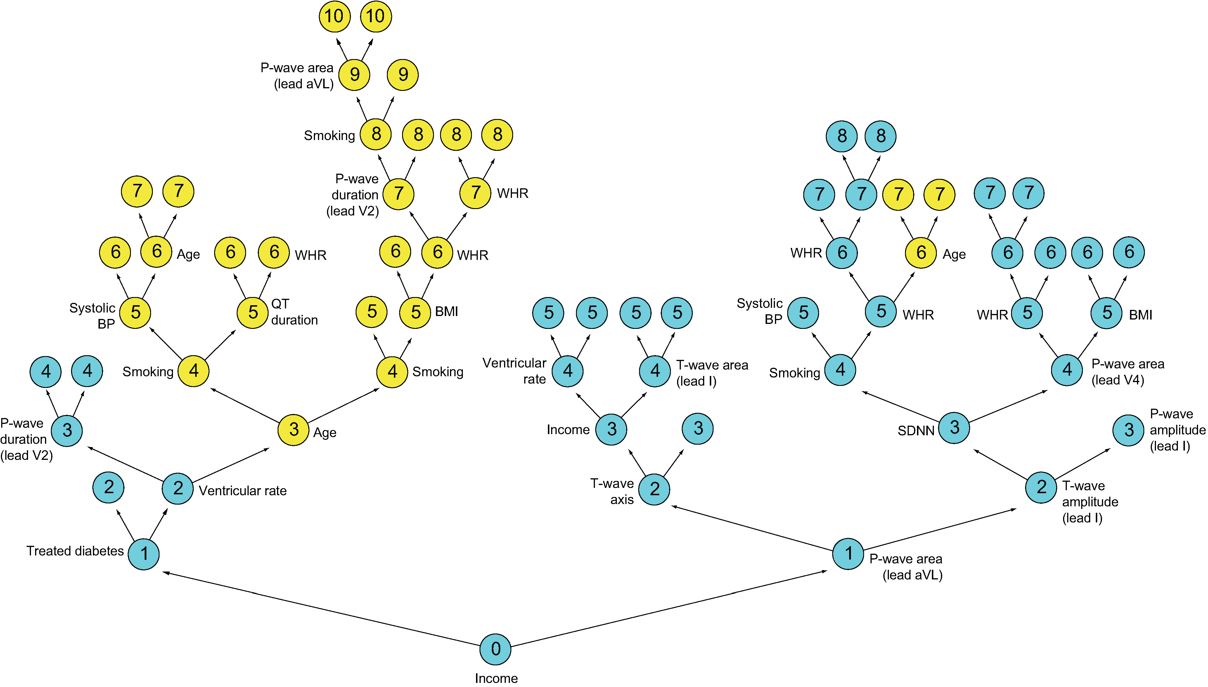
Figure 1 illustrates minimal depth. Shown is a single tree highlighting the two variables “Income” and “Age” and their maximal subtrees from a survival analysis involving cardiovascular patients (note that the tree has been inverted with the root node displayed at the bottom). Maximal subtrees are indicated by color; node depth is indicated by an integer located in the center of a tree node. The root node is split using Income; thus its maximal subtree (in blue) is the entire tree and its minimal depth is 0. For Age, there are two maximal subtrees (in yellow) on each side of the tree, with depths 3 and 6, with the closest to the root node being on the left. For Age, the minimal depth is 3.

Figure 1

Illustration of minimal depth. The depth of a node, \(d\), is the distance to the root node (depicted here at the bottom of the tree). Therefore, \(d\in\{0,1,\ldots,D(T)\}\), where \(D(T)\) is the depth of a tree, defined as the distance from the root node to the farthest terminal node. For this tree, \(D(T)=10\) and the first split at depth \(d=0\) (the root node) is on the variable Income. Click to zoom in.

Denote the minimal depth for a variable \(v\) by \(D_v\). In high-dimensional sparse settings under the assumption that \(v\) is noisy (i.e., a variable with no signal), it can be shown [1] that for \(0\le d\le D(T)-1\), where \(D(T)\) is the depth of a tree \(T\), \[ \mathbb{P}\Biggl\{D_v=d\,\Bigl|\, \ell_0,\ldots,\ell_{D(T)}, \text{$v$ is noisy}\Biggr\} = \left[1-\left(1-\frac{1}{p}\right)^{\ell_d}\right] \prod_{j=0}^{d-1}\left(1-\frac{1}{p}\right)^{\ell_j}, \] where \(\ell_d\) equals the number of non-terminal nodes at depth \(d\) and \(p\) is the number of variables. To ensure that probabilities sum to 1, define \[\begin{eqnarray*} &&\mathbb{P}\Biggl\{D_v=D(T)\,\Bigl|\, \ell_0,\ldots,\ell_{D(T)}, \text{$v$ is noisy}\Biggr\}\\ &&\qquad = 1-\sum_{d=0}^{D(T)-1} \mathbb{P}\Biggl\{D_v=d\,\Bigl|\, \ell_0,\ldots,\ell_{D(T)}, \text{$v$ is noisy}\Biggr\}. \end{eqnarray*}\]

Minimal Depth Thresholding

Having a simple closed form expression for the minimal depth distribution is useful as it allows us to characterize the properties of minimal depth. The mean of this distribution, called the mean minimal depth, is used as a threshold value for selecting variables, with those variables exceeding the threshold being identified as noisy. These are removed from the model.

Notice that in order to calculate mean minimal depth, we need to substitute values for the parameters \(\ell_d\) and \(D(T)\) into the minimal depth distribution. There are two ways to do this that leads to sensible values for mean minimal depth. The first method uses tree-averaged estimates to approximate the parameters. Thus, if \(\overline{\ell}_d\) and \(\overline{D}\) are the tree-averaged estimates of \(\ell_d\) and \(D(T)\), the forest averaged minimal depth threshold is approximated by \[ \mathbb{E}\left[D_v\Bigl|\, \overline{\ell}_0,\ldots,\overline{\ell}_{\overline{D}}, \text{$v$ is noisy}\right]. \] This was the method used by Ishwaran et al. [1, 2].

A second approach is to take the tree average of the mean minimal depth threshold, where for each tree, the mean of the distribution is calculated by substituting tree values for \(\ell_d\) and \(D(T)\). Thus, using a subscript of \(b\) to indicate dependence on the tree \(T_b\), the forest averaged minimal depth threshold is \[ \frac{1}{B}\sum_{b=1}^B \mathbb{E}\left[D_v\Bigl|\, \ell_{0,b},\ldots,\ell_{D(T_b)}, \text{$v$ is noisy}\right]. \] This method tends to produce slightly larger threshold values than the method above. Both methods are available in the function max.subtree() which calculates minimal depth and threshold values and is implemented in the package. Users can select between the two strategies using the option conservative.

p-Asymptotics: Problems with Minimal Depth

Unfortunately, without some additional supervision, minimal depth variable selection will have subpar performance in high dimensions. This is because there is a subtle relationship involving \(p\), the depth of a tree, \(D(T)\), and the right tail of the distribution of minimal depth that effects minimal depth selection in high dimensions. Even when the underlying model is sparse, it becomes impossible to grow a tree deep enough to properly select variables as \(p\rightarrow\infty\). This motivates several strategies for regularizing minimal depth variable selection [1, 2].

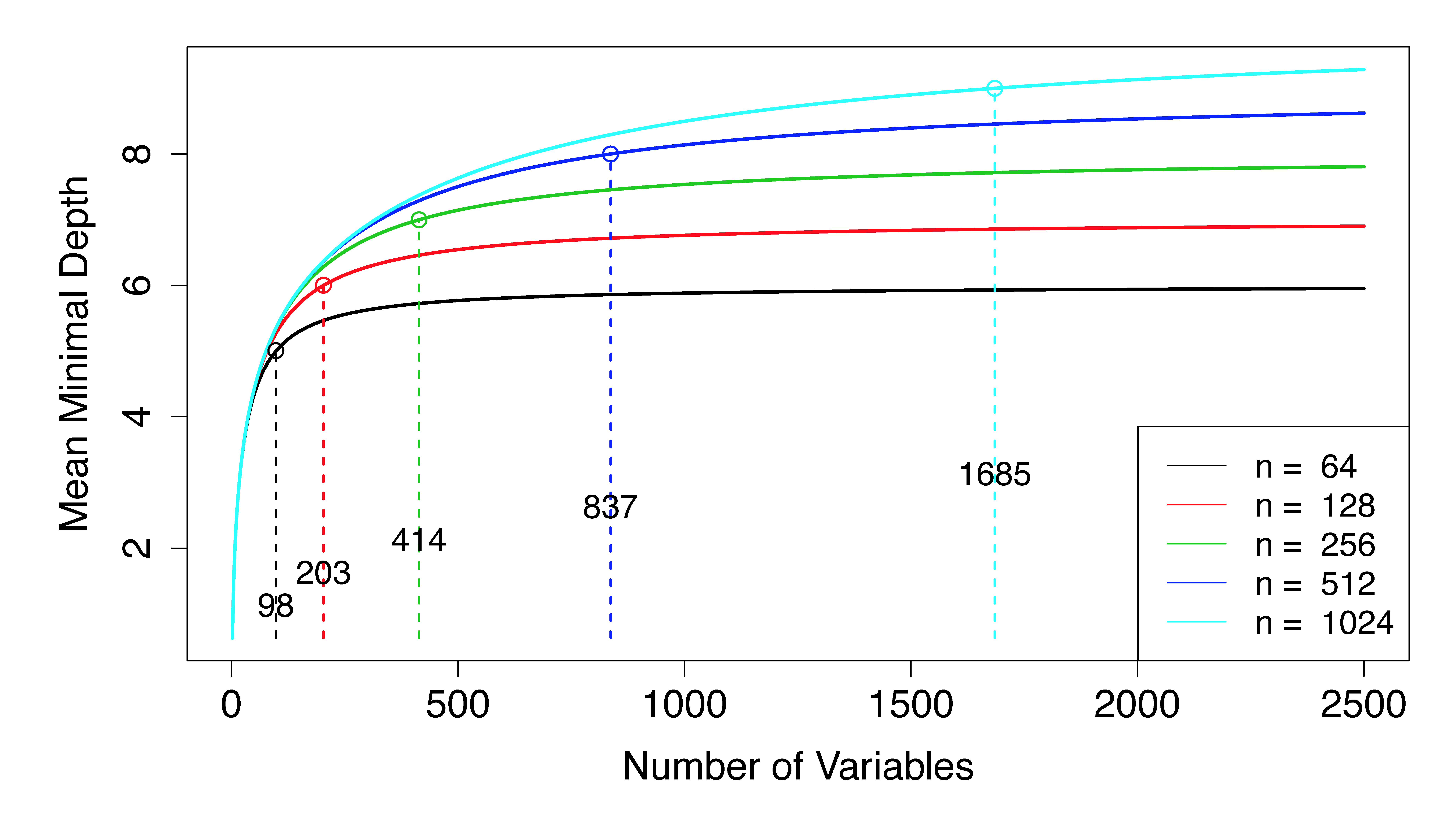
This limiting degeneracy of minimal depth is illustrated in Figure 2. The figure displays the mean minimal depth, \(\mathbb{E}(D_v)\), as a function of \(p\) assuming \(v\) is a noisy variable and that the tree \(T\) is balanced (i.e., \(\ell_d=2^d\)). The mean minimal depth converges to the maximal depth of a tree, \(D(T)\), as \(p\) increases. The vertical lines and superimposed integers in the figure indicate the number of variables at which point the mean exceeds \(D(T) - 1\). As can be seen, this can occur quite rapidly. For example, with a sample size of \(n=256\), only \(p=414\) variables are required. Indeed, regardless of the sample size, it appears that the number of variables required is \(O(n)\).

Figure 2

Mean minimal depth under the assumption a variable \(v\) is noisy assuming a balanced tree. Dashed vertical lines and superimposed integers indicate the number of variables at which point the mean exceeds \(D(T)-1\). Click to zoom in.

To understand why Figure 2 happens, we can rewrite the minimal depth distribution as \[ \mathbb{P}\Biggl\{D_v=d\,\Bigl|\, \ell_0,\ldots,\ell_{D(T)}, \text{$v$ is noisy}\Biggr\} = \left[1-\left(1-\frac{1}{p}\right)^{l_d}\right]\left(1-\frac{1}{p}\right)^{L_d}, \] for \(0\le d\le D(T)-1\) where \(L_d=\ell_0+\cdots+\ell_{d-1}\). Under the assumption of a balanced tree, we have \(L_d=1+2+\cdots+2^{d-1}=\ell_d-1\). Therefore, if \(p\gg \ell_{D(T)}\), the above probability is of order \[\begin{eqnarray*} \left[\frac{\ell_d}{p}+o(\ell_d/p)\right]\left[1-\frac{\ell_{d}-1}{p}+o(\ell_{d}/p)\right] &=&\frac{\ell_d}{p}\left(1-\frac{\ell_d-1}{p}\right)+o(\ell_d/p)\\ &\le& \frac{\ell_{D(T)}}{p}+o(1/p)=o(1). \end{eqnarray*}\] Therefore, all probabilities are near zero and minimal depth will start to coalesce around the depth of the tree, \(D(T)\).

Illustration

The \(p\)-asymptotics just described assumes a balanced tree which is unrealistic in high-dimensional sparse settings. Trees are generally unbalanced in such scenarios due to several factors, including the end-cut preference property of trees [4] which has a strong effect in sparse problems. This unbalancedness will help to improve minimal depth to some extent, and the probabilities given above may be slightly better. Nevertheless, we have observed that without some form of supervision, minimal depth will quickly start to plateau in high dimensions and become ineffective.

The following example illustrates a simple solution to improve minimal depth. We use the microarray data set used by [5] for developing a breast cancer gene expression signature. Here the data contains 4707 expression values on 78 patients with survival information.

In our first approach, we run RSF and calculate minimal depth the usual way (without any supervision).

## ------------------------------------------------------------
## minimal depth with/without supervision
## van de Vijver Microarray Breast Cancer data 
## ------------------------------------------------------------
library("randomForestSRC")

## load the microarray data set
data(vdv, package = "randomForestSRC")

## calculate minimal depth as usual (without supervision)
o <- rfsrc(Surv(Time, Censoring) ~ ., vdv)
md <- max.subtree(o)$order[, 1]

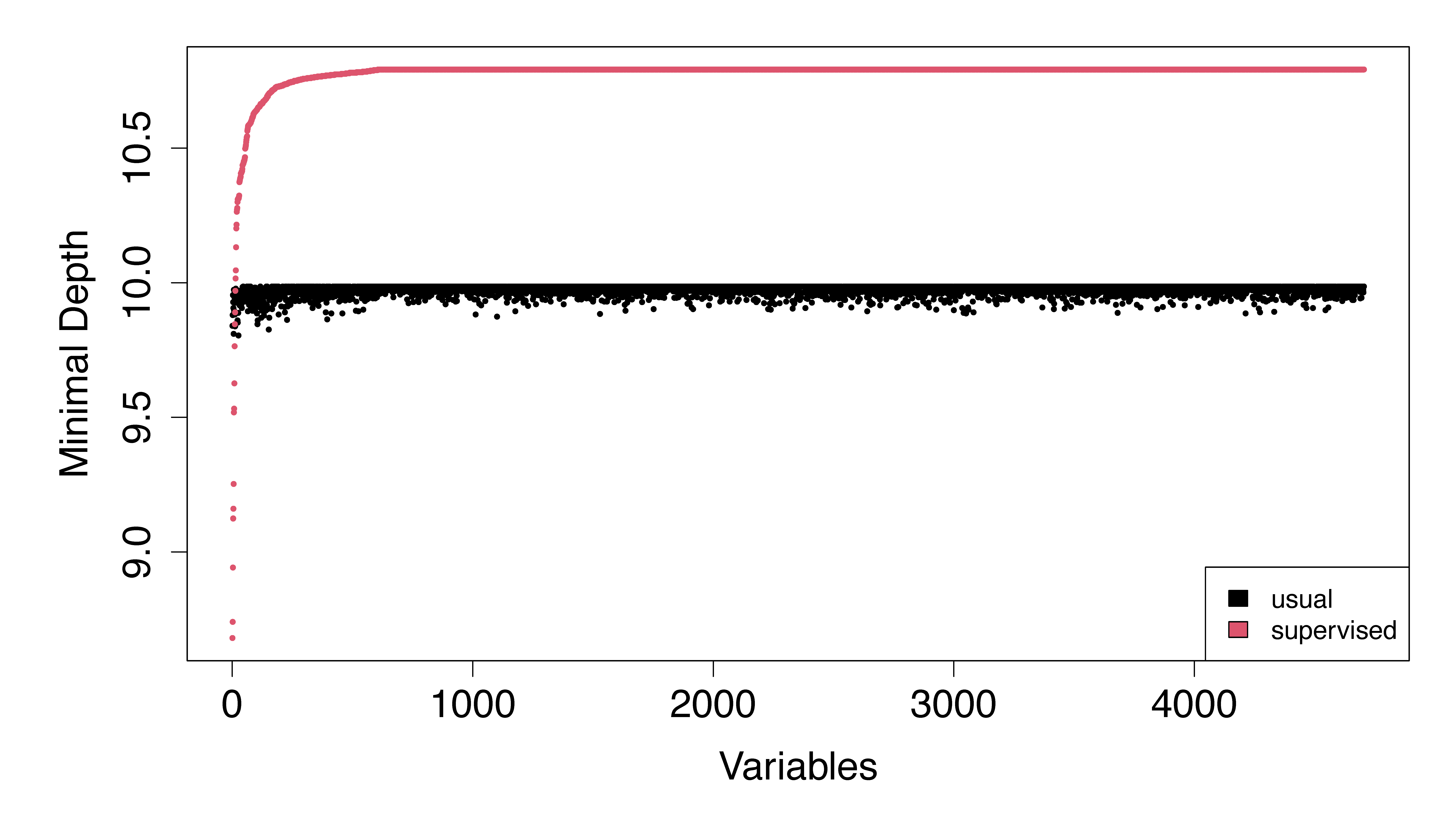
In our second improved approach, we run a pilot forest and keep track of total number of times a variable is used to split a node. Random feature selection is turned off. Then we run RSF with feature selection probabilities guided by the splitting strength of a variable obtained from the pilot run. Notice in Figure 3 how minimal depth values are now significantly improved compared with the values without supervision. The latter are nearly constant, just as expected by our \(p\)-asymptotics.

## run survival trees and calculate number of times each variable splits a node
xvar.used <- rfsrc(Surv(Time, Censoring) ~ ., vdv, nodedepth = 6,
                   var.used="all.trees", mtry = Inf, nsplit = 100)$var.used

## calculate minimal depth with supervision
## use number of times variable splits to guide random feature selection
os <- rfsrc(Surv(Time, Censoring) ~ ., vdv, xvar.wt = xvar.used)
mds <- max.subtree(os)$order[, 1]


## compare usual minimal depth to supervised minimal depth
matplot(cbind(md, mds)[order(mds),], pch=16, cex=.5, ylab="minimal depth", xlab="variables")
legend("bottomright", legend = c("usual", "supervised"), fill = 1:2)

Figure 3

Second-Order Maximal Subtrees

As discussed, maximal subtrees are a powerful tool for exploring the importance of a variable using the concept of minimal depth. We have so far considered first-order maximal subtrees, but second-order maximal subtrees are another type of maximal subtree useful for exploring variable relationships [6]. A second-order maximal \((w,v)\)-subtree is a maximal \(w\)-subtree within a maximal \(v\)-subtree for a variable \(v\). A variable \(w\) having a maximal \((w,v)\)-subtree close to the root of \(v\) will be highly associated with \(v\) because \(w\) splits closely after \(v\). By considering the minimal depth of \(w\) for its maximal \((w,v)\)-subtrees we can quantify the association of \(w\) with \(v\).

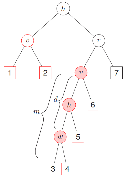
To illustrate this, consider the two maximal \(v\)-subtrees in Figure 4, marked in red. The maximal \(v\)-subtree on the left side is with terminal nodes 1 and 2; that on the right side is with terminal nodes 3, 4, 5, and 6. Let \(T_{v,w}\) be the second-order maximal \((w,v)\)-subtree of the maximal subtree \(T_v\). The minimal depth from \(v\) to \(w\) in \(T_{v}\) equals the distance from the root node of \(T_{v}\) to the root of the closest second order maximal \((w,v)\)-subtree \(T_{v,w}\), which is denoted as \(D_{v,w}\). Let \(m\) be the depth of subtree \(T_{v,w}\) and let \(D(T)\) be the depth of the entire tree \(T\). Assuming \(v\) and \(w\) are weak variables and independent with each other, we have

\[\begin{equation}\label{dvw} \mathbb{P}\{D_{v,w}=d\}=\sum_{m=d}^{D(T)}\mathbb{P}\{D_v=D(T)-m\}\mathbb{P}\{D_w=D(T)-m+d\}. \end{equation}\]

Figure 4

As illustrated by Figure 4, the interaction between variables \(v\) and \(w\) is marked with pink background: when these two variables interact with each other, we expact this depth to be smaller and this close split pattern to be repeated frequently among different trees. A single tree can be used to calculate multiple minimal depths of variables in multiple maximal subtrees, such as variables \(h\) and \(v\) in Figure 4, where the maximal \(h\)-subtree is the entire tree. The minimal depth \(D_{v,w}=d\) is normalized by the depth of the corresponding subtree as \(d/m\) and normalized values from different maximal \(v\)-subtrees are averaged across the entire forest. This normalized index ranges from 0 to 1 and smaller values indicate stronger interaction effects.

Illustration of Second-Order Maximal Subtrees

Set sub.order=TRUE in max.subtree() to obtain the minimal depth of a variable relative to another variable. This returns a \(p\times p\) matrix, where \(p\) is the number of variables, and entries \((i,j)\) are the normalized relative minimal depth of a variable \(j\) within the maximal subtree for variable \(i\), where normalization adjusts for the size of \(i\)’s maximal subtree. Entry \((i,i)\) is the normalized minimal depth of \(i\) relative to the root node. The matrix should be read by looking across rows (not down columns) and identifies interrelationship between variables. Small \((i,j)\) entries indicate interactions. See find.interaction() in our Manual for more contents.

library("randomForestSRC")
mtcars.obj <- rfsrc(mpg ~ ., data = mtcars[, 1:7])
v.max <- max.subtree(mtcars.obj, sub.order=TRUE)
v.max$sub.order

>            cyl      disp        hp      drat        wt      qsec
> cyl  0.6863333 0.9608333 0.9586667 0.9811667 0.9685000 0.9893333
> disp 0.9640000 0.6298333 0.9376667 0.9795000 0.9608333 0.9850000
> hp   0.9775000 0.9598333 0.6806667 0.9833333 0.9616667 0.9930000
> drat 0.9933333 0.9811667 0.9828333 0.8711667 0.9825000 0.9963333
> wt   0.9595000 0.9393333 0.9548333 0.9845000 0.6258333 0.9795000
> qsec 0.9956667 0.9946667 0.9923333 0.9943333 0.9953333 0.9398333

Cite this vignette as
H. Ishwaran, X. Chen, A. J. Minn, M. Lu, M. S. Lauer, and U. B. Kogalur. 2021. “randomForestSRC: minimal depth vignette.” http://randomforestsrc.org/articles/minidep.html.

@misc{HemantMinimal,
    author = "Hemant Ishwaran and Xi Chen and Andy J. Minn and Min Lu and Michael S. Lauer 
              and Udaya B. Kogalur",
    title = {{randomForestSRC}: minimal depth vignette},
    year = {2021},
    url = {http://randomforestsrc.org/articles/minidep.html},
    howpublished = "\url{http://randomforestsrc.org/articles/minidep.html}",
    note = "[accessed date]"
}

References

1. Ishwaran H, Kogalur UB, Gorodeski EZ, Minn AJ, Lauer MS. High-dimensional variable selection for survival data. Journal of the American Statistical Association. 2010;105:205–17.

2. Ishwaran H, Kogalur UB, Chen X, Minn AJ. Random survival forests for high-dimensional data. Statistical Analysis and Data Mining: The ASA Data Science Journal. 2011;4:115–32.

3. Ishwaran H, Lu M, Kogalur UB. randomForestSRC: Variable importance (VIMP) with subsampling inference vignette. 2021. http://randomforestsrc.org/articles/vimp.html.

4. Ishwaran H. The effect of splitting on random forests. Machine Learning. 2015;99:75–118.

5. Van’t Veer LJ, Dai H, Van De Vijver MJ, He YD, Hart AA, Mao M, et al. Gene expression profiling predicts clinical outcome of breast cancer. Nature. 2002;415:530–6.

6. Lu M, Sha Y, Silva T, Colaprico A, Sun X, Ban Y, et al. LR hunting: A random forest based cell-cell interaction discovery method for single-cell gene expression data. Frontiers in Genetics. 2021;12:1431. https://www.frontiersin.org/article/10.3389/fgene.2021.708835.