Variable Importance (VIMP) with Subsampling Inference
Hemant Ishwaran
Min Lu
Udaya B.
Kogalur
2026-03-26
vimp.Rmd
Introduction
Random forests (RF) software developed by [1] provides for various options for calculating variable importance (VIMP). One approach used for classification forests is Gini impurity importance [2]. However, by far, the more popular measure of importance is another measure provided by the software, called permutation importance (referred to as Breiman-Cutler importance). Unlike Gini importance which estimates importance using in-sample impurity, permutation importance adopts a prediction based approach by using prediction error attributable to the variable. A clever feature is that rather than using cross-validation, which is computationally expensive for forests, permutation importance estimates prediction error by making use of out-of-bootstrap cases. Recall each tree is calculated from a bootstrap sample of the original data. The approximately left from the bootstrap represents out-of-sample data which can be used for estimating prediction performance. This data is called out-of-bag (OOB) and prediction error obtained from it is called OOB error [3, 4]. Permutation importance permutes a variable’s OOB data and compares the resulting OOB prediction error to the original OOB prediction error — the motivation being that a large positive value indicates a variable with predictive importance.
Permutation (Breiman-Cutler) Importance
In the OOB cases for a tree, randomly permute all values of the
th
variable. Put these new covariate values down the tree and compute a new
internal error rate. The amount by which this new error exceeds the
original OOB error is defined as the importance of the
th
variable for the tree. Averaging over the forest yields VIMP.
—
Measure 1 (Manual On Setting Up, Using, And Understanding Random Forests
V3.1
Mathematical description of VIMP
In a nutshell, we can see that permutation importance is essentially a technique for estimating the importance of a variable by comparing performance of the estimated model with and without the variable in it. This is a very popular technique and has been used throughout machine learning [2, 5–14].
One technical point we should mention though, is that permutation importance does not actually remove the variable from the model, and this is one of the unique features of it that makes it computationally fast. What actually happens is that the permutation is designed to push a variable to a terminal node different than its original assignment. Essentially, the farther away this is from the original terminal node, the more likely it is that the variable is important. The following figure illustrates this.
Figure 1
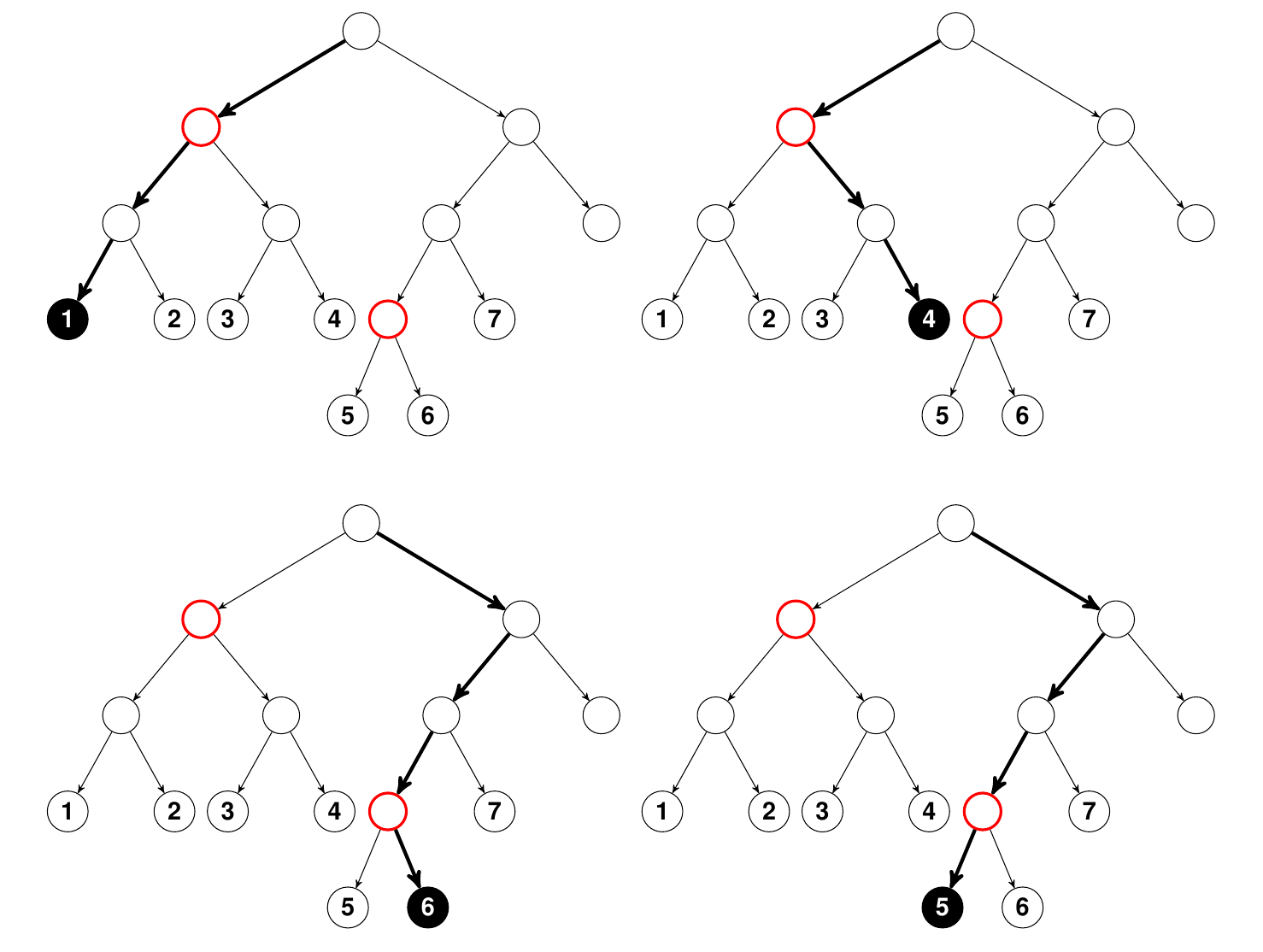
Illustration of how randomly permuting a variable leads to
different terminal node assignments. Nodes colored red are tree nodes
that split on the target variable
.
In the top panel on the left using bold arrows is the path that a data
point ${\bf x}$ takes as it traverses
through the tree to its terminal node assignment “1”. On the right, the
coordinate of ${\bf x}$ has been
randomly permuted and its new terminal node assignment is now “4”. In
the bottom panel is the path for another ${\bf
x}$ value. Its terminal node assignment is “6”. However when
is permuted, its new terminal assigment becomes “5”. Importantly, notice
that in the top panel the terminal node assignment after randomly
permuting
is much farther than its original terminal node assignment than in the
bottom panel. This shows that the higher variable
splits in the tree, the more an effect permutation has on final terminal
node membership, and hence on prediction error. Click to zoom in.
Notation
The fact that permutation importance is a comparison of model performance under alteration to the variable can be seen more clearly as we now provide a more formal description of VIMP (hereafter we will refer to Breiman-Cutler importance simply as VIMP). We assume is the response and ${\bf X}\in\mathscr{X}$ is the -dimensional feature where can be continuous, binary, categorical, or survival, and ${\bf X}$ can be continuous or discrete. We assume the underlying problem involves a nonparametric regression framework where the goal is to estimate a functional $\psi({\bf x})$ of the response given ${\bf X}={\bf x}$. Estimation is based on the learning data $\mathscr{L}_n=\{({\bf X}_1,Y_1),\ldots,({\bf X}_n,Y_n)\}$, where $({\bf X}_i,Y_i)$ are independently distributed with the same distribution as $({\bf X},Y)$.
Examples of $\psi({\bf x})$ are:
- The conditional mean $\psi({\bf x})=\mathbb{E}[Y|{\bf X}={\bf x}]$ in regression.
- The conditional class probabilities $\psi_1({\bf x}),\ldots,\psi_C({\bf x})$ in a -multiclass problem, where $\psi_c({\bf x})=\mathbb{P}\{Y=c|{\bf X}={\bf x}\}$, for .
- The survival function $\psi({\bf x})=\mathbb{P}\{T^o>t|{\bf X}={\bf x}\}$ in survival analysis. Here represents the bivariate response comprised of the observed survival time and censoring indicator , where are the unobserved event and censoring times.
RF predictor
Recall our getting started vignette [15] that a RF is a collection of randomized tree predictors . Here $\varphi({\bf x},{\Theta}_m,\mathscr{L}_n)$ denotes the th random tree predictor of $\psi({\bf x})$ and are independent identically distributed random quantities encoding the randomization needed for constructing a tree. Note that each is selected prior to growing the tree and is independent of the learning data, .
The tree predictors are combined to form the finite forest estimator of $\psi({\bf x})$, $$ \varphi({\bf x},{\Theta}_1,\ldots,{\Theta}_M,\mathscr{L}_n) = \frac{1}{M} \sum_{m=1}^M \varphi({\bf x},{\Theta}_m,\mathscr{L}_n). $$ The infinite forest estimator is obtained by taking the limit as and equals $$ \varphi({\bf x},\mathscr{L}_n) = \mathbb{E}_{\Theta}\left[ \varphi({\bf x},{\Theta},\mathscr{L}_n)\right]. \label{forest.pred.infinite} $$
Loss function
Calculating VIMP assumes some well defined notion of prediction error. Therefore, we assume there is an appropriately prechosen loss function used to measure performance of a predictor in predicting . Examples include:
- Squared error loss in regression problems.
- For classification problems, measures of performance used are the misclassification error or the Brier score. For the latter, , where is the estimator for the conditional probability .
- For survival, the weighted Brier score [16, 17] can be used (see our RSF vignette, [18]).
Tree VIMP
Let be the th bootstrap sample and let be the OOB data. Write ${\bf X}=(X^{(1)},\ldots,X^{(p)})$ where denotes the th feature coordinate. The permuted value of the th coordinate of is denoted by . Substituting this into the th coordinate of ${\bf X}$ yields $\tilde{{\bf X}}^{(j)}$: $$ \tilde{{\bf X}}^{(j)}=(X^{(1)},\ldots,X^{(j-1)},\tilde{X}^{(j)},X^{(j+1)},\ldots,X^{(p)}). $$ VIMP is calculated by taking the difference in prediction error under the original ${\bf X}$ to prediction error under the perturbed $\tilde{{\bf X}}^{(j)}$ over OOB data. More formally, let denote the VIMP for for the th tree. It follows that $$\begin{eqnarray*} && I(X^{(j)},{\Theta}_m,\mathscr{L}_n)\\ && \qquad = \frac{\sum_{i\in\mathscr{L}_n^{\text{OOB}}({\Theta}_m)} \ell(Y_i, \varphi(\tilde{{\bf X}}^{(j)}_i,{\Theta}_m,\mathscr{L}_n))}{|\mathscr{L}_n^{\text{OOB}}({\Theta}_m)|} - \frac{\sum_{i\in\mathscr{L}_n^{\text{OOB}}({\Theta}_m)} \ell(Y_i, \varphi({\bf X}_i,{\Theta}_m,\mathscr{L}_n))}{|\mathscr{L}_n^{\text{OOB}}({\Theta}_m)|}. \end{eqnarray*}$$
VIMP
Averaging tree VIMP over the forest yields VIMP: An infinite tree estimator for VIMP can be defined analogously by taking the limit as , It is worth noting that neither of these definitions explicitly use the forest ensemble predictor and instead each relies on single tree predictors. This is a unique feature of VIMP because it is a tree-based estimator of importance.
Illustration
VIMP can be extracted using the option importance in
either grow mode using rfsrc() or in prediction mode using
predict.rfsrc(). The default importance is Breiman-Cutler
and is specified by setting importance=TRUE or more
directly by importance = "permute". There is also a
dedicated interface vimp() for calculating VIMP.
Below we use the Iris data set to illustrate VIMP for the multiclass
problem. For classification, the default setting used by the package is
misclassification error which corresponds to zero-one loss for the loss
function. Performance under the Brier score is also available. To
request VIMP for the Brier score use the option
perf.type="brier".
We note that the package uses a slightly modified Brier score, which we refer to as the normalized Brier score and is defined as follows. Let be the response. If denotes the predicted probability that equals class , , the normalized Brier score is defined as Observe how the normalizing constant used here is different than the value typically used for the Brier score. We multiply the traditional Brier score by because we have noticed that the value for the Brier score under random guessing depends on the number of classes, . If increases, the Brier score under random guessing converges to 1. The normalizing constant used here resolves this problem and yields a value of 1 for random guessing, regardless of . Thus, anything below 1 signifies a classifier that is better than pure guessing. A perfect classifier has value 0. In the output given below for the Iris analysis, the Brier score and the normalized Brier score are listed in line 14 and 15. The OOB AUC value (area under the ROC curve) is listed in line 16.
The OOB confusion matrix for the analysis is listed from line 19 to 25. Overall misclassification error equals sum of off-diagonal elements of the confusion matrix divided by total sample size, and is displayed on line 27. The overall misclassification error, along with the misclassification errors for each specific class label, are displayed in line 17.
library(randomForestSRC)
iris.obj <- rfsrc(Species ~ ., data = iris)
iris.obj

> 1                           Sample size: 150
> 2             Frequency of class labels: 50, 50, 50
> 3                       Number of trees: 500
> 4             Forest terminal node size: 1
> 5         Average no. of terminal nodes: 9.52
> 6  No. of variables tried at each split: 2
> 7                Total no. of variables: 4
> 8         Resampling used to grow trees: swor
> 9      Resample size used to grow trees: 95
> 10                             Analysis: RF-C
> 11                               Family: class
> 12                       Splitting rule: gini *random*
> 13        Number of random split points: 10
> 14                    (OOB) Brier score: 0.02479567
> 15         (OOB) Normalized Brier score: 0.11158052
> 16                            (OOB) AUC: 0.99306667
> 17                     (OOB) Error rate: 0.04666667, 0.02, 0.06, 0.06
> 18
> 19 Confusion matrix:
> 20
> 21             predicted
> 22   observed   setosa versicolor virginica class.error
> 23   setosa         49          0         0        0.02
> 24   versicolor      0         47         3        0.06
> 25   virginica       0          3        47        0.06
> 26
> 27   Overall (OOB) error rate: 4.666667%
Use the vimp() function:
print(vimp(iris.obj)$importance)

>                       all     setosa  versicolor    virginica
> Sepal.Length 0.0091442229 0.04457982  0.02392088  0.005436564
> Sepal.Width  0.0001288857 0.02065894 -0.01848432 -0.001087313
> Petal.Length 0.2012338277 0.74154728  0.54256905  0.340328885
> Petal.Width  0.2386940818 0.90790613  0.67304658  0.346852761
The above output lists misclassification error VIMP for each predictor. First column is overall VIMP, remaining columns are class specific VIMP for “setosa”, “versicolor” and “virginica” obtained by conditioning the data on the respective class labels.
# VIMP using brier prediction error
print(vimp(iris.obj, perf.type = "brier")$importance)

>                     all     setosa  versicolor    virginica
> Sepal.Length 0.03569896 0.01235568 0.030889279 0.0214482610
> Sepal.Width  0.01093318 0.01034908 0.009094997 0.0003689035
> Petal.Length 0.44634242 0.25745261 0.309862352 0.2415413527
> Petal.Width  0.49537671 0.30815849 0.347015242 0.2425419476
The above output lists Brier score VIMP for each predictor. First column is overall VIMP, remaining columns are class specific VIMP for “setosa”, “versicolor” and “virginica” obtained by conditioning the data on the respective class labels.
Inference for VIMP
Now we describe how to estimate the variance for VIMP and construct confidence regions [19]. So far we have the following constructs: Notice that we have changed our notation slightly, replacing with and with . This will be advantageous as not only does it simplify the notation, but it also helps emphasize that the quantities involved are estimators, which makes it easier to conceptualize and state results about their properties.
For the theoretical derivation, it will be easier to deal with infinite tree VIMP, , rather than Monte Carlo VIMP, . The latter obviously closely approximates the former for a large enough number of trees. Our goal is to approximate the distribution of the rescaled test statistic and this in turn will be used to approximate the variance of and for constructing confidence intervals.
Bootstrap variance estimator (.164 estimator)
When stated this way, a first thought that might come to mind, is why not just use the bootstrap variance estimator? Recall that the bootstrap is used for approximating the distribution for complicated estimators and this approximation naturally provides an estimate for the variance as well.
More formally, let be i.i.d. random values with common distribution . Let be some estimator for , an unknown real-valued parameter we wish to estimate. The bootstrap estimator for the variance of is based on the following simple idea. Let be the empirical measure for the data. Let be a bootstrap sample obtained by independently sampling points from , i.e. Because converges to under general conditions, we should expect the moments of the bootstrap estimator to closely approximate population values, which should therefore closely approximate if the estimator is converging. In particular where denote bootstrap estimators from independently drawn boootstrap samples.
However, there is a problem with using the bootstrap variance estimator for VIMP. A direct application cannot be used due to a double-bootstrap effect. This is because if we use the bootstrap method, then this forces us to grow a collection of forests, where each forest is constructed using a given bootstrap data. But each bootstrap contains duplicates and when we construct a tree, which also bootstraps the data, then we are bootstrapping a bootstrap data set, which compromises the coherence of the OOB data.
We can see that the double bootstrap data lowers the probability of being truly OOB. Let be the number of occurrences of case in , where is a bootstrap sample of the data. Then, We have Hence, $$\begin{eqnarray*} &&\hskip-50pt \sum_{l=1}^n \Pr\{\text{$i$ is truly OOB in $\mathscr{L}_n^{\text{IB}}({\Theta})$}|n_i=l\} \,\Pr\{n_i=l\}\\ && =\sum_{l=1}^n \left(\frac{n-l}{n}\right)^n\Pr\{n_i=l\}\\ && \asymp \sum_{l=1}^n \left(\frac{n-l}{n}\right)^n \left(\frac{\text{e}^{-1}1^l}{l!}\right)\\ && \text{e}^{-1}\sum_{l=1}^n \left(1-\frac{l}{n}\right)^n\frac{1}{l!}\\ && \asymp \text{e}^{-1}\sum_{l=1}^n \frac{\text{e}^{-l}}{l!} \asymp .1635 < .368. \end{eqnarray*}$$ Therefore, double bootstrap data has an OOB size of which is smaller than the true OOB size of .
The above discussion points to a simple solution to the problem which we call the .164 bootstrap estimator [19]. The .164 estimator is a bootstrap variance estimator but is careful to use only truly OOB data. The algorithm for this procedure is outlined by the following steps:
- Draw a bootstrap sample .
- Calculate Monte Carlo VIMP using uniquified OOB data
- Repeat times obtaining estimators .
- Estimate the variance of VIMP by
Subsampling (sampling without replacement)
A problem with the .164 bootstrap estimator is that its OOB data set is smaller than a typical OOB estimator (16.4% versus 36.8%). Thus in a forest of 1000 trees, the .164 estimator uses about 164 trees on average to calculate VIMP for a case compared with 368 trees used in a standard calculation. This can reduce efficiency of the .164 estimator. Another problem is computational expense. The .164 estimator requires repeatedly fitting RF to bootstrap data which can be computationally intensive, especially for big data.
To avoid these problems, we propose a more efficient procedure based on subsampling theory [20]. The idea rests on calculating VIMP over small i.i.d. subsets of the data. Because sampling is without replacement, this avoid ties in the OOB data that creates problems for the bootstrap. Also, because each forest is grown for a very small data set, the procedure is computationally efficient.
To explain this approach abstractly, as before let be i.i.d. random values with common distribution and let be some estimator for some unknown parameter . Let be the entire collection of subsets of of size . For each , let be the subsampled estimator. The goal will be to use estimators to approximate the sampling distribution of , the rescaled test statistic defined by
Let
denote the distribution of
.
If
and
[20]
The expression on the left,
,
closely approximates
which is a
-statistic
of order
from which the distributional result follows by
-statistic
theory. Now the assumption
implies due to i.i.d. sampling that
where the last line follows by the
assumption that
is asymptotically smaller than
.
This last line is the most important, since unlike the previous two
lines it does not depend on the unknown parameter. Thus it can be
calculated, and the strategy is to approximate
using
calculated from subsampled estimators as the last line shows these
converge to the true
which is the limiting distribution for
.
Subsampling estimator for the variance of VIMP
Let be different subsampled sets from and let denote the learning data for a subsampled set . The subsampled estimator for the variance is [19] $$ \hat{\upsilon}^{(j)}_{n,b}= \frac{b/n}{K} \sum_{k=1}^K \Bigl(\hat{\theta}^{(j)}_{n,b,s_k} - \frac{1}{K}\sum_{k'=1}^K \hat{\theta}^{(j)}_{n,b,s_{k'}}\Bigr)^2 $$ where is the subsampled Monte Carlo VIMP estimator. It is instructive to compare this to the bootstrap estimator where . We see that the estimators are essentially doing the same thing but the difference between them is in the method of sampling. The bootstrap uses sampling with replacement whereas the subsampled estimator uses sampling without replacement. Also the subsample size is asympotically smaller than . This is the reason for the scaling factor appearing above, which is another difference between the estimators.
Delete-d jackknife estimator for the variance of VIMP
The subsampling variance estimator is closely related to the delete- jackknife [21]. The delete- estimator works on subsets of size and for VIMP is defined as [19] $$ \hat{\upsilon}^{(j)}_{n,J(d)} = \frac{r/d}{K}\sum_{k=1}^K (\hat{\theta}^{(j)}_{n,r,s_k} - \hat{\theta}^{(j)}_{n,M})^2, \hskip10pt r=n-d. $$ Setting (which means ), and with rearrangement, $$\begin{eqnarray*} \hat{\upsilon}^{(j)}_{n,J(d)} &=& \overbrace{\frac{b/(n-b)}{K}}^{\color{red}{\asymp b/n}} \sum_{k=1}^K \Bigl(\hat{\theta}^{(j)}_{n,b,s_k} - \frac{1}{K}\sum_{k'=1}^K\hat{\theta}^{(j)}_{n,b,s_{k'}}\Bigr)^2\\ &&+ \frac{b}{n-b} \Bigl( \underbrace{\frac{1}{K}\sum_{k=1}^K \hat{\theta}^{(j)}_{n,b,s_k}-\hat{\theta}^{(j)}_{n,M}}_{\color{red}{\text{bias}}} \Bigr)^2 . \end{eqnarray*}$$
The first term closely approximates the subsampling estimator since , while the second term is a bias correction to the subsampled estimator. This correction is due to the fact the subsampled estimator tries to approximate the Monte Carlo VIMP using subsampled Monte Carlo estimators. Furthermore, this correction is always upwards because the bias term is squared and always positive.
Confidence regions
Subsampling can also be used to calculate nonparametric confidence intervals [20]. The general idea for constructing a confidence interval for a target parameter is as follows. Define the quantile for the subsampling distribution as . Similarly, define the quantile for the limiting distribution of as . Then, assuming and , the interval contains with asymptotic probability if is a continuity point of .
While the above is able to calculate a nonparametric confidence interval for VIMP, a more practicable and stable solution can be obtained by assuming asympotic normality. Let be population VIMP defined earlier. Let be an estimator for . Assuming asymptotic normality, an asymptotic confidence region for , the true VIMP, can be defined as where is the -quantile from a standard normal, . We have found that the assumption of asymptotic normality is quite reasonable in most applications [19].
Illustration
The following R code calculates the confidence interval using
delete-
jackknife estimator. For .164 confidence intervals, we can use
subsample(iris.obj, B = 25, bootstrap = TRUE).
library(randomForestSRC)
iris.obj <- rfsrc(Species ~ ., data = iris)
## very small sample size so need largish subratio
reg.smp.o <- subsample(iris.obj, B = 25, subratio = .5)
## summary of results
print(reg.smp.o)

> ===== VIMP confidence regions for all  =====
> nonparametric:
>       Sepal.Length Sepal.Width Petal.Length Petal.Width
> 2.5%         2.388       0.303       24.857      28.376
> 25%          3.182       1.196       27.343      31.846
> 50%          3.823       1.348       28.000      33.578
> 75%          4.172       1.454       28.863      35.219
> 97.5%        4.726       1.840       31.238      36.439
> parametric:
>       Sepal.Length Sepal.Width Petal.Length Petal.Width
> 2.5%         2.534       0.526       24.212      27.527
> 25%          3.381       1.001       26.446      30.528
> 50%          3.825       1.251       27.618      32.102
> 75%          4.270       1.500       28.790      33.676
> 97.5%        5.117       1.976       31.024      36.676
> parametric (jackknife):
>       Sepal.Length Sepal.Width Petal.Length Petal.Width
> 2.5%         2.522       0.535       24.156      27.021
> 25%          3.377       1.004       26.427      30.353
> 50%          3.825       1.251       27.618      32.102
> 75%          4.274       1.497       28.809      33.850
> 97.5%        5.129       1.967       31.080      37.183

> ===== VIMP confidence regions for setosa  =====
> nonparametric:
>       Sepal.Length Sepal.Width Petal.Length Petal.Width
> 2.5%        -0.371      -0.105       26.974      34.992
> 25%          1.613       1.159       28.220      36.268
> 50%          2.766       1.420       29.050      37.237
> 75%          3.289       1.682       29.742      37.914
> 97.5%        4.289       2.051       31.707      39.335
> parametric:
>       Sepal.Length Sepal.Width Petal.Length Petal.Width
> 2.5%         1.143       0.282       26.454      33.403
> 25%          2.904       1.074       28.187      35.000
> 50%          3.827       1.490       29.096      35.838
> 75%          4.751       1.905       30.006      36.676
> 97.5%        6.512       2.697       31.739      38.273
> parametric (jackknife):
>       Sepal.Length Sepal.Width Petal.Length Petal.Width
> 2.5%         0.063       0.252       26.496      32.279
> 25%          2.532       1.064       28.202      34.613
> 50%          3.827       1.490       29.096      35.838
> 75%          5.123       1.916       29.991      37.063
> 97.5%        7.592       2.728       31.697      39.397

> ===== VIMP confidence regions for versicolor  =====
> nonparametric:
>       Sepal.Length Sepal.Width Petal.Length Petal.Width
> 2.5%         1.278      -0.424       21.287      30.080
> 25%          3.111       0.658       23.704      32.393
> 50%          3.464       0.997       25.058      34.299
> 75%          4.618       1.396       27.871      35.745
> 97.5%        5.368       1.956       32.149      39.395
> parametric:
>       Sepal.Length Sepal.Width Petal.Length Petal.Width
> 2.5%         0.670       0.007       18.824      26.436
> 25%          2.135       0.822       22.887      29.950
> 50%          2.903       1.250       25.019      31.793
> 75%          3.672       1.678       27.151      33.637
> 97.5%        5.137       2.494       31.214      37.150
> parametric (jackknife):
>       Sepal.Length Sepal.Width Petal.Length Petal.Width
> 2.5%         0.270      -0.090       18.665      24.360
> 25%          1.997       0.789       22.832      29.235
> 50%          2.903       1.250       25.019      31.793
> 75%          3.809       1.712       27.206      34.351
> 97.5%        5.537       2.591       31.374      39.226

> ===== VIMP confidence regions for virginica  =====
> nonparametric:
>       Sepal.Length Sepal.Width Petal.Length Petal.Width
> 2.5%         2.498       1.010       21.559      12.851
> 25%          4.147       1.446       25.683      24.405
> 50%          4.685       1.569       27.666      28.219
> 75%          5.792       1.800       30.619      30.018
> 97.5%        6.709       2.052       33.912      33.216
> parametric:
>       Sepal.Length Sepal.Width Petal.Length Petal.Width
> 2.5%         2.130       0.396       21.372      17.174
> 25%          3.821       0.792       26.025      24.508
> 50%          4.708       1.000       28.466      28.357
> 75%          5.595       1.208       30.907      32.206
> 97.5%        7.286       1.604       35.560      39.541
> parametric (jackknife):
>       Sepal.Length Sepal.Width Petal.Length Petal.Width
> 2.5%         2.182      -0.265       21.455      16.987
> 25%          3.839       0.565       26.053      24.444
> 50%          4.708       1.000       28.466      28.357
> 75%          5.577       1.436       30.879      32.270
> 97.5%        7.234       2.266       35.477      39.727

## plot confidence regions using the delete-d jackknife variance estimator
#plot.subsample(reg.smp.o)
Figure 2
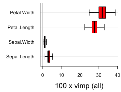
In the above output, parametric refers to inference under the assumption of asymptotic normality, while nonparametric refers to the nonparametric subsampling method described in the Section on Confidence regions. Figure 2 displays the confidence regions using the delete-d jackknife.
Cite this vignette as
H. Ishwaran, M. Lu, and
U. B. Kogalur. 2021. “randomForestSRC: variable importance (VIMP) with
subsampling inference vignette.” http://randomforestsrc.org/articles/vimp.html.
@misc{HemantVIMP,
    author = "Hemant Ishwaran and Min Lu and Udaya B. Kogalur",
    title = {{randomForestSRC}: variable importance {(VIMP)} with subsampling inference vignette},
    year = {2021},
    url = {http://randomforestsrc.org/articles/vimp.html},
    howpublished = "\url{http://randomforestsrc.org/articles/vimp.html}",
    note = "[accessed date]"
}