AUC Splitting for Multiclass Problems

Introduction

The receiver operating characteristic curve (ROC curve) is a popular method for performance evaluation of a classifier. Originally it was developed for assessing the accuracy of a test for predicting disease [1] and we will discuss it first in this context. The ROC curve for a test $Z$ is the plot of the true positive rate (sensitivity) versus the false positive rate (1 - specificity) of the dichotomized variable $Z_{\tau}=I\{Z>\tau\}$ as $\tau\in\mathbb{R}$ is varied over all possible values for $Z$. The curve characterizes all possible trade-off’s between sensitivity and specificity for the test. The trace of the curve lies in the square $[0,1]\times[0,1]$: the higher the curve is above the $y=x$ line within this square, the more accurate the test $Z$ is in delineating between disease states. The overall accuracy of the test can be measured by the area under the curve (AUC), where area is computed using the trapezoidal rule. This summary value is an estimate of the probability that two randomly selected individuals, one diseased and the other non-diseased, are correctly ranked by the test [1] (see the Appendix for a proof). Thus the AUC for the ROC curve has the interesting interpretation that it measures ranking performance of a test. For this reason, AUC is often used as a metric for assessing performance of a classifier in machine learning.

To see how this applies to classification, let $Y_1,\ldots,Y_n$ denote the binary response variables. For consistency with the ROC literature, we assume $Y=0$ is the non-diseased group and $Y=1$ is the diseased group. Denote by $Z$ the predicted value from the machine learning classifier. Let $\mathbb{P}_n(\cdot)=n^{-1}\sum_{i=1}^n I\{(Z_i,Y_i)\in\cdot\}$ be the empirical measure for $(Z_1,Y_1),\ldots,(Z_n,Y_n)$. The ROC curve is the plot of \[\begin{eqnarray} \text{ROC}(\tau) &=& \left(\text{False Positive Rate}(\tau), \text{True Positive Rate}(\tau)\right)\\ &=& \left(1 - \text{Specificity}(\tau), \text{Sensitivity}(\tau)\right)\\ &=& \Bigl(\mathbb{P}_n\{Z>\tau|Y=0\},\mathbb{P}_n\{Z>\tau|Y=1\}\Bigr), \end{eqnarray}\] as $\tau$ varies over all possible values for $Z_1,\ldots,Z_n$.

In fact, letting $\tau_1<\tau_2<\cdots<\tau_m$ represent the set of all unique $Z$ values, and setting $\tau_0=-\infty$, the ROC curve is the interpolated curve of the points $\text{ROC}(\tau_k)$, $k=0,\ldots,m$. The AUC is the area bounded between this interpolated curve and the horizontal line $\{(x,0): 0\le x\le 1\}$. Thus,

(1)

\[\begin{eqnarray} \text{AUC} &=&\int_{-\infty}^\infty\mathbb{P}_n\{Z>\tau|Y=1\}\,\mathbb{P}_n\{Z>d\tau|Y=0\}\nonumber\\ &=&\frac{1}{2}\sum_{k=0}^{m-1}(\alpha_k-\alpha_{k+1})(\beta_k+\beta_{k+1}), \label{AUC.trapezoidal} \end{eqnarray}\] where $\alpha_k=\mathbb{P}_n\{Z>\tau_k|Y=0\}$ and $\beta_k=\mathbb{P}_n\{Z>\tau_k|Y=1\}$.

AUC splitting rule

Now we show how this can be used for tree splitting. To describe a fast AUC splitting rule we will require a closed form expression for the ROC curve and its area. Without loss of generality consider splitting the root node. Let $L$ and $R$ denote the left and right-daughter nodes resulting from this split. We can summarize the frequency of obsevations in the daughter nodes using the following $2\times2$ table (Table 1).

Table 1

Frequency of cases in left and right daughter nodes by disease status.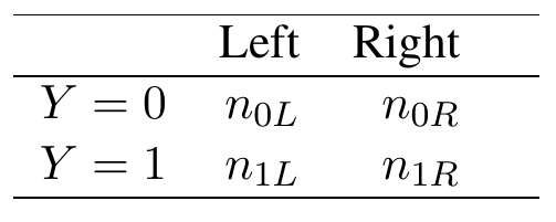

Here $Z$ predicts $Y=1$. There can be at most two distinct values of $Z$, one for each daughter node: \[ \tau_1=\frac{n_{1L}}{n_L}\hskip5pt\text{($Z$ values of left node)}, \hskip10pt \tau_2=\frac{n_{1R}}{n_R}\hskip5pt\text{($Z$ values of right node)}, \] where $n_L,n_R$ are the sample sizes for the left and right daughters ($n_L+n_R=n$; $n_{0L}+n_{1L}=n_L$; $n_{0R}+n_{1R}=n_R$). The ROC curve is therefore \[ \text{ROC}(\tau) = \Bigl(\mathbb{P}_n\{Z>\tau|Y=0\},\mathbb{P}_n\{Z>\tau|Y=1\}\Bigr) \] as $\tau$ varies over $\tau=\tau_1,\tau_2$.

To derive the AUC it will be helpful to break up the calculation into three cases: $\tau_1>\tau_2$, $\tau_1<\tau_2$ and $\tau_1=\tau_2$. Consider the first case $\tau_2>\tau_1$. Because the predicted value for the left daughter node is $\tau_1$, it is not possible for $Z>\tau$ for $Z\in L$ when $\tau=\tau_1$. Therefore \[ \text{ROC}(\tau_1) = \Bigl(\mathbb{P}_n\{Z>\tau_1,Z\in R\,|Y=0\},\mathbb{P}_n\{Z>\tau_1, Z\in R\,|Y=1\}\Bigr). \] Now because all $Z$ in $R$ are larger than $\tau_1$ by assumption, we have

(2)

\[ \text{ROC}(\tau_1)=\Bigl(\frac{n_{0R}}{n_{0L}+n_{0R}}, \frac{n_{1R}}{n_{1L}+n_{1R}}\Bigr). \label{case.1} \] Furthermore, because it is not possible for $Z>\tau_2$ due to the assumption $\tau_2$ is the largest observed value, we have $\text{ROC}(\tau_2)=(0,0)$. Therefore the ROC curve contains only three points, $(0,0)$, $\text{ROC}(\tau_1)$ and $(1,1)$.

Now consider the second case when $\tau_2<\tau_1$. When $\tau=\tau_1$, it is not possible for $Z>\tau$ as $\tau$ is the largest observed value and therefore $\text{ROC}(\tau_1)=(0,0)$. When $\tau=\tau_2<\tau_1$ it is not possible for $Z>\tau$ for $Z\in R$; hence \[ \text{ROC}(\tau_2) = \Bigl(\mathbb{P}_n\{Z>\tau_2,Z\in L\,|Y=0\},\mathbb{P}_n\{Z>\tau_2, Z\in L\,|Y=1\}\Bigr). \] Now because all $Z$ in $L$ are larger than $\tau_2$ because $\tau_1>\tau_2$, we have

(3)

\[ \text{ROC}(\tau_2)=\Bigl(\frac{n_{0L}}{n_{0L}+n_{0R}}, \frac{n_{1L}}{n_{1L}+n_{1R}}\Bigr). \label{case.2} \] Therefore the ROC curve contains only three points, $(0,0)$, $\text{ROC}(\tau_2)$ and $(1,1)$.

Finally, consider the third case $\tau_1=\tau_2$. Because it is not possible for $Z>\tau$ when $\tau=\tau_1=\tau_2$, it follows that $R(\tau_1)=R(\tau_2)=(0,0)$ and consequently the ROC curve contains only two points, $(0,0)$ and $(1,1)$.

To work out the AUC let us visit each of the three above cases. For (2), let \[ (\alpha,\beta)=\Bigl(\frac{n_{0R}}{n_{0L}+n_{0R}}, \frac{n_{1R}}{n_{1L}+n_{1R}}\Bigr). \] Then the area under the curve equals the area under the curve for the three points $(0,0)$, $(\alpha,\beta)$, $(1,1)$, which equals \[\begin{eqnarray} &&\hskip-20pt \frac{1}{2}\alpha\beta+(1-\alpha)\beta+ \frac{1}{2}(1-\alpha)(1-\beta)\\ &&=\frac{1}{2}\alpha\beta+\beta-\alpha\beta+ \frac{1}{2}(1-\alpha-\beta+\alpha\beta)\\ &&=\frac{1}{2}(1-\alpha+\beta). \end{eqnarray}\] Now for the second case (3), notice that \[ (1-\alpha,1-\beta)=\Bigl(\frac{n_{0L}}{n_{0L}+n_{0R}}, \frac{n_{1L}}{n_{1L}+n_{1R}}\Bigr). \] Therefore, the ROC curve is comprised of the three points $(0,0)$, $(1-\alpha,1-\beta)$, $(1,1)$. The AUC is therefore \[\begin{eqnarray} &&\hskip-20pt \frac{1}{2}(1-\alpha)(1-\beta)+\alpha(1-\beta) + \frac{1}{2}\alpha\beta\\ &&=\frac{1}{2}(1-\alpha-\beta+\alpha\beta)+\alpha-\alpha\beta+ \frac{1}{2}\alpha\beta\\ &&=\frac{1}{2}(1-\beta+\alpha). \end{eqnarray}\] Observe that this is different than the first case. Finally, for the third case, since there are only two points $(0,0)$ and $(1,1)$ on the ROC curve, the AUC must equal $1/2$.

By symmetry, the AUC should not depend on the labeling of the terminal nodes and therefore the AUC for $Z$ is defined to be the maximum value of the three cases \[ \max\left(\frac{1}{2}(1-\alpha+\beta),\, \frac{1}{2}(1-\beta+\alpha), \frac{1}{2}\right) = \max\left(\frac{1}{2}(1-\alpha+\beta),\, \frac{1}{2}(1-\beta+\alpha)\right), \] where the right-hand side follows since an AUC of $1/2$ implies $\alpha=\beta$ and because the maximum of $(1-\alpha+\beta)$ and $(1-\beta+\alpha)$ can never be less than $1$.

Implementation of the AUC splitting rule

It is now a simple matter to implement the AUC splitting rule. For a proposed split into left and right daugther nodes $L$ and $R$, calculate \[ (\alpha,\beta)=\Bigl(\frac{n_{0R}}{n_{0L}+n_{0R}}, \frac{n_{1R}}{n_{1L}+n_{1R}}\Bigr). \] The split-statistic is \[ \theta(L,R) = \max\left(\frac{1}{2}(1-\alpha+\beta),\, \frac{1}{2}(1-\beta+\alpha)\right). \] Choose the split yielding the {} split-statistic value $\theta(L,R)$.

Connection to random forests quantile classification

There is connection between maximizing the AUC splitting rule and the recently proposed RFQ (random forests quantile classification) method of [2]. The latter approach is motivated by maximizing the sum of the true negative rate (TNR) and the true positive rate (TPR).

By symmetry, we can consider the first term $(1-\alpha+\beta)$ appearing in the AUC splitting rule $\theta(L,R)$, \[\begin{eqnarray} (1-\alpha+\beta) &:=& 1-\mathbb{P}_n\{Z>\tau|Y=0\}+\mathbb{P}_n\{Z>\tau|Y=1\}\\ &=& \text{Specificity}(\tau)+\text{Sensitivity}(\tau)\\ &=& 1-\text{False Positive Rate}(\tau)+ \text{True Positive Rate}(\tau)\\ &=& \text{True Negative Rate}(\tau)+ \text{True Positive Rate}(\tau). \end{eqnarray}\] We can conclude that maximizing the AUC splitting rule is equivalent to RFQ’s goal of maximizing TNR$+$TPR.

Extension to the multiclass setting

Now we describe the AUC splitting rule for the multiclass setting by building on the two-class AUC splitting rule. Now the response $Y$ can take one of $K>2$ distinct values, $Y\in\{1,\ldots,K\}$. The interpretation for the diagnostic test $Z$ is also different. Following a proposed split to a tree node, the diagnostic test $Z$ predicts $Y=k_2$ versus $Y=k_1$ for all possible $k_1\ne k_2$. To take into account all these comparisons, the AUC is defined as the average over all $k_1<k_2$ comparisons [3].

More formally, we summarize the frequencies resulting from the tree node split as a $K\times 2$ table. Given there are $K$ classes and two nodes, we have $2K$ predicted probabilities that $Z$ is evaluated over: \[ \text{left node:}\hskip5pt \tau_L^{(1)}=\frac{n_{1L}}{n_L},\, \tau_L^{(2)}=\frac{n_{2L}}{n_L},\,\cdots, \tau_L^{(K)}=\frac{n_{KL}}{n_L}. \] \[ \text{right node:}\hskip5pt \tau_R^{(1)}=\frac{n_{1R}}{n_R},\, \tau_R^{(2)}=\frac{n_{2R}}{n_R},\,\cdots, \tau_R^{(K)}=\frac{n_{KR}}{n_R}. \] See Table 2 for illustration.

Table 2

Left: Frequency of cases. Right: Predicted probabilities for left and right daughter nodes for the $K>2$ multiclass setting.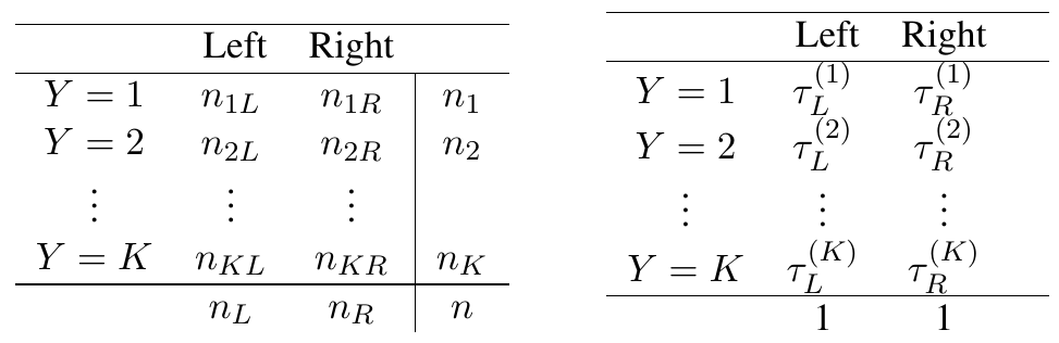

For each $k_1<k_2$ comparison, we can treat $k_1$ as the baseline “no-disease” case and $k_2$ as the “disease” case. Define \[ (\alpha_{k_1,k_2},\beta_{k_1,k_2})=\Bigl(\frac{n_{k_1R}}{n_{k_1}}, \frac{n_{k_2R}}{n_{k_2}}\Bigr). \] Define the following U-statistics \[ U_{k_1,k_2} = \frac{1}{2}\left(1 - \alpha_{k_1,k_2} + \beta_{k_1,k_2}\right),\hskip10pt U_{k_2,k_1} = \frac{1}{2}\left(1 - \beta_{k_1,k_2} + \alpha_{k_1,k_2}\right). \] Using a similar argument as before, the AUC for the comparison between $k_1$ and $k_2$ is \[ \text{AUC}_{k_1,k_2}= \max\left(U_{k_1,k_2}, U_{k_2,k_1}\right). \] The AUC for the proposed split is defined as the average over all $k_1<k_2$ comparisons. Thus, \[\begin{eqnarray} \text{AUC} &=& \frac{2}{K(K-1)}\sum_{k_1<k_2} \text{AUC}_{k_1,k_2}\\ &=& \frac{2}{K(K-1)}\sum_{k_1<k_2} \max\left(U_{k_1,k_2}, U_{k_2,k_1}\right). \end{eqnarray}\]

Implementation of the AUC multiclass splitting rule

It is now a simple matter to implement the AUC multiclass splitting rule. For a proposed split into left and right daugther nodes $L$ and $R$, calculate the $K\times 2$ frequencies as in Table 2. Using these, calculate $U_{k_1,k_2}$ and $U_{k_2,k_1}$ for all $k_1< k_2$. The split-statistic is \[ \theta(L,R) = \frac{2}{K(K-1)}\sum_{1\le k_1<k_2\le K} \max\left(U_{k_1,k_2}, U_{k_2,k_1}\right). \] Choose the split yielding the maximum split-statistic value $\theta(L,R)$.

Appendix: Connection to the Mann-Whitney U-statistic

We show that the AUC is directly related to the Mann-Whitney U-statistic. Although this is a well known result [1], it is helpful to provide an independent proof of this fact.

Let $(Z_{i,0})_{i=1}^{n_0}$ denote the set of test values having class label $Y=0$. Also let $(Z_{j,1})_{j=1}^{n_1}$ be those test values with $Y=1$. Note that $n_0+n_1=1$. Define \[ S(Z_{i,0},Z_{j,1})=\left\{ \begin{array}{ll} 0 &\mbox{if $Z_{i,0}>Z_{j,1}$}\\ 1/2 &\mbox{if $Z_{i,0}=Z_{j,1}$}\\ 1 &\mbox{if $Z_{i,0}<Z_{j,1}$}. \end{array}\right. \] The Mann-Whitney U-statistic is

(4)

\[ U=\frac{1}{n_0 n_1}\sum_{i=1}^{n_0}\sum_{j=1}^{n_1} S(Z_{i,0},Z_{j,1}). \label{MW.U} \] By definition (4), we can see that $U$ estimates the probability of correctly ranking two individuals randomly selected from the two disease groups: \[ U=\mathbb{P}_n\{Z_{i,0}<Z_{j,1}\}. \] The AUC, however, has no such obvious interpretation. Theorem 1 given below makes this connection.

Theorem 1: The AUC defined by (1) equals the Mann-Whitney U-statistic (4).

By definition, $\alpha_k-\alpha_{k+1}=\mathbb{P}_n\{Z=\tau_{k+1}|Y=0\}$. Consequently, by (1) \[\begin{eqnarray} \text{AUC} &=&\frac{1}{2}\sum_{k=0}^{m-1} \beta_k\times\mathbb{P}_n\{Z=\tau_{k+1}|Y=0\}\\ &&\qquad\qquad +\frac{1}{2}\sum_{k=0}^{m-1} \beta_{k+1}\times\mathbb{P}_n\{Z=\tau_{k+1}|Y=0\}. \end{eqnarray}\] The following is a key identity needed for the proof.
For each $k=0,\ldots,m-1$, \[\begin{eqnarray} &&\beta_k\times\mathbb{P}_n\{Z=\tau_{k+1}|Y=0\}\\ &&\qquad = \frac{1}{n_0 n_1}\sum_{Z_{i,0}=\tau_{k+1}}\sum_{j=1}^{n_1} I\{Z_{j,1}>\tau_k\}\\ &&\qquad = \frac{1}{n_0 n_1}\sum_{Z_{i,0}=\tau_{k+1}}\sum_{j=1}^{n_1} \Bigl(I\{Z_{j,1}>Z_{i,0}\}+I\{Z_{j,1}=Z_{i,0}\}\Bigr)\\ &&\qquad = \frac{1}{n_0 n_1}\sum_{Z_{i,0}=\tau_{k+1}} \sum_{j=1}^{n_1}\left(S(Z_{i,0},Z_{j,1})+\frac{1}{2}I\{Z_{j,1}=Z_{i,0}\}\right). \end{eqnarray}\] By similar reasoning we have another key identity, \[\begin{eqnarray} &&\beta_{k+1}\times\mathbb{P}_n\{Z=\tau_{k+1}|Y=0\}\\ &&\qquad = \frac{1}{n_0 n_1}\sum_{Z_{i,0}=\tau_{k+1}}\sum_{j=1}^{n_1} I\{Z_{j,1}>Z_{i,0}\}\\ &&\qquad = \frac{1}{n_0 n_1}\sum_{Z_{i,0}=\tau_{k+1}} \sum_{j=1}^{n_1}\left(S(Z_{i,0},Z_{j,1})-\frac{1}{2}I\{Z_{j,1}=Z_{i,0}\}\right). \end{eqnarray}\] Deduce that \[\begin{eqnarray} \text{AUC} &=&\frac{1}{n_0 n_1}\sum_{k=0}^{m-1}\sum_{Z_{i,0}=\tau_{k+1}} \sum_{j=1}^{n_1} S(Z_{i,0},Z_{j,1})\\ &=&\frac{1}{n_0 n_1}\sum_{k=1}^m\sum_{Z_{i,0}=\tau_k} \sum_{j=1}^{n_1} S(Z_{i,0},Z_{j,1}). \end{eqnarray}\] It is easily seen that the right-hand side is (4).

Cite this vignette as
H. Ishwaran, M. Lu, and U. B. Kogalur. 2022. “randomForestSRC: AUC splitting for multiclass problems vignette.” http://randomforestsrc.org/articles/aucsplit.html.

@misc{HemantAUCsplit,
    author = "Hemant Ishwaran and Min Lu and Udaya B. Kogalur",
    title = {{randomForestSRC}: {AUC} splitting for multiclass problems vignette},
    year = {2022},
    url = {http://randomforestsrc.org/articles/aucsplit.html},
    howpublished = "\url{http://randomforestsrc.org/articles/aucsplit.html}",
    note = "[accessed date]"
}

References

1. Hanley JA, McNeil BJ. The meaning and use of the area under a receiver operating characteristic (ROC) curve. Radiology. 1982;143:29–36.

2. O’Brien R, Ishwaran H. A random forests quantile classifier for class imbalanced data. Pattern recognition. 2019;90:232–49.

3. Hand DJ, Till RJ. A simple generalisation of the area under the ROC curve for multiple class classification problems. Machine Learning. 2001;45:171–86.

Hemant Ishwaran

Min Lu

Udaya B. Kogalur

2023-05-29

Introduction

(1)

AUC splitting rule

Table 1

(2)

(3)

Implementation of the AUC splitting rule

Connection to random forests quantile classification

Extension to the multiclass setting

Table 2

Implementation of the AUC multiclass splitting rule

Appendix: Connection to the Mann-Whitney U-statistic

(4)

References

AUC Splitting for Multiclass Problems

Hemant Ishwaran Min Lu Udaya B. Kogalur

2023-05-29

Introduction

(1)

AUC splitting rule

Table 1

(2)

(3)

Implementation of the AUC splitting rule

Connection to random forests quantile classification

Extension to the multiclass setting

Table 2

Implementation of the AUC multiclass splitting rule

Appendix: Connection to the Mann-Whitney U-statistic

(4)

References

Hemant Ishwaran

Min Lu

Udaya B. Kogalur