sidClustering
Hemant Ishwaran
Alejandro Mantero
Min Lu
Udaya B. Kogalur
2023-05-29
sidClustering.Rmd
Introduction
Machine learning is generally divided into two branches: supervised and unsupervised learning. In supervised learning the response is known and the goal is to train a model to predict its value, while in unsupervised learning the response is unknown and the general goal is to find structure in the feature data. This makes the problem more difficult. Another challenge in unsupervised learning occurs when data have a mix of both numerical as well as categorical feature variables (referred to as mixed data). Such data is very common in modern big data settings such as in medical and health care problems. However many unsupervised methods are better suited for data with only continuous variables. Our goal is to construct an unsupervised procedure capable of handling the scenario of mixed data.
One strategy of unsupervised algorithms involves reworking the problem into a supervised classification problem [1, 2]. Breiman’s unsupervised method [3] is one widely known random forests (RF) method which uses this strategy. The idea is to generate an artificial dataset that goes into the model along side the original data. A RF classifier is trained on the data formed by combining the original data (class label 1) and artificial data (class label 2) and the proximity matrix is extracted from the resulting forest. Then standard clustering techniques can be utilized on the proximity matrix such as hierarchical clustering [4] or partitioning about medoids [5] to determine clusters (for convenience we refer to these techniques as HC and PAM, respectively).
Although Breiman’s clustering method has been demonstrated to work well, it is highly dependent on the distribution chosen for the artificial data class. Therefore, we have introduced a new RF method for unsupervised learning which we call sidClustering [6]. This new method is based on two new concepts: (1) sidification of the data (we call this new enhanced feature space, SID for staggered interaction data); (2) multivariate random forests (MVRF) [7]. The latter is applied to the sidified data to develop distance between points via the multivariate relationship between features and their two-way interactions. The sidClustering algorithm is implmemented in the package by the self-titled function, sidClustering(). For completeness, the function also provides an implementation of Breiman clustering using the two data mode generation schemes described in [8]. An illustration of sidClustering() is given at the end.
sidClustering algorithm
We use \({\bf X}=(X_1,\ldots,X_d)^T\) to represent the \(d\)-dimensional feature. The learning data equals the set of features \(\mathscr{L}=({\bf X}_i)_{i=1}^n\) observed for \(n\) cases. Algorithm 1 sidClustering describes the sidClustering algorithm. Line 2 creates the enhanced feature space from the sidification of the data. Line 3 fits a MVRF using the SID main features as response values and the SID interaction features as the predictors. The distance matrix between points obtained from the multivariate regression are extracted in Line 4 and then converted to Euclidean distance in Line 5. Clusters are then obtained in Line 6 by applying either HC or PAM using the Euclidean distance based on the RF distance matrix obtained in line 4.
Algorithm 1 sidClustering
1: procedure sidClustering \(\mathscr{L}=({\bf X}_{i})_{i=1}^n\)
2: \(\quad\) Sidify the original variables (see Algorithm 2 Sidification), obtaining the sidified data, \(\mathscr{L}^S=({\bf Z}_i,{\bf Y}_i)_{i=1}^n\)
3: \(\quad\) Use SID interaction features \(({\bf Z}_i)_{i=1}^n\) to predict SID main features \(({\bf Y}_i)_{i=1}^n\) using MVRF
4: \(\quad\) Extract RF distance from the trained multivariate forest
5: \(\quad\) Calculate Euclidean distance on the matrix of distances
6: \(\quad\) Cluster the observations based on distance of Step 5 utilizing HC or PAM
7: end procedure
The key idea behind sidClustering is to turn the unsupervised problem into a multivariate regression problem. The multivariate outcomes are denoted by \({\bf Y}=(Y_1,\ldots,Y_d)^T\) and are called the SID main effects. The \({\bf Y}\) are obtained by shifting the original \({\bf X}\) features by making them strictly positive and staggering them so their ranges are mutually exclusive (we think of this process as ``staggering’’). For example, suppose \(X_j\) and \(X_k\) are coordinates of \({\bf X}\) which are continuous. Then the SID main effects obtained from \(X_j\) and \(X_k\) are coordinates \(Y_j\) and \(Y_k\) of \({\bf Y}\) defined by \[ Y_j=\delta_j+X_j,\hskip10pt Y_k=\delta_k+X_k, \] where \(\delta_j,\delta_k>0\) are real values suitably chosen so that \(Y_j,Y_k\) are positive and the range of \(Y_j\) and \(Y_k\) do not overlap. The features used in the multivariate regression are denoted by \({\bf Z}\) and are called the SID interaction features. The SID interaction features are obtained by forming all pairwise interactions of the SID main effects, \({\bf Y}\). Thus for the example above, the SID interaction corresponding to features \(X_j\) and \(X_k\) is some coordinate of \({\bf Z}\) denoted by \(X_j\star X_k\) and defined to be the product of \(Y_j\) and \(Y_k\) \[ X_j\star X_k = Y_j \times Y_k = (\delta_j+X_j)(\delta_k+X_k). \] The staggering of \(Y_j\) and \(Y_k\) so that their ranges do not overlap will ensure identification between the SID interactions \({\bf Z}\) (which are the features in the multivariate regression) and the SID main effects \({\bf Y}\) (which are the outcomes in the mulivariate regression).
The reason for using sidified data in the multivariate regression tree approach is as follows. Because \({\bf Y}\) is directly related to \({\bf X}\), informative \({\bf X}\) features will be cut by their SID interactions \({\bf Z}\) because this bring about a decrease in impurity in \({\bf Y}\) (and hence \({\bf X}\)). This then allows cluster separation, because if coordinates of \({\bf X}\) are informative for clusters, then they will vary over the space in a systematic manner. As long as the SID interaction features \({\bf Z}\) are uniquely determined by the original features \({\bf X}\), cuts along \({\bf Z}\) will be able to find the regions where the \({\bf X}\) informative features vary by cluster, thereby not only reducing impurity, but also separating the clusters which are dependent on those features.
RF distance
Line 4 of the sidClustering algorithm makes use of a new forest distance. This new distance is used in place of the usual proximity measure used by RF. Similar to proximity, the goal of the new distance is to measure dissimilarity between observations, however unlike proximity it does not use terminal node membership for assessing closeness of data points. Instead, it uses a measurement of distance based on the tree topology to provide a more sensitive measurement. The issue with proximity is that if two observations split far down the tree versus close to the root node, both scenarios are counted as having a proximity of zero, even though the first scenario involves data points closer in the sense of the tree topology.
Let \(T_b\) denote the \(b\)th tree in a forest. The forest distance is applied to SID interaction features \({\bf Z}\) (as these serve as the features in the MVRF). For each pair of observed data points \({\bf Z}_i\) and \({\bf Z}_j\), define \(S({\bf Z}_i,{\bf Z}_j,T_b)\) to equal the minimum number of splits on the path from the terminal node containing \({\bf Z}_i\) to the terminal node containing \({\bf Z}_j\) in \(T_b\) such that the path includes at least one common ancestor node of \({\bf Z}_i\) and \({\bf Z}_j\). Similarly, define \(R({\bf Z}_i,{\bf Z}_j,T_b)\) as the minimum number of splits on the path from the terminal node containing \({\bf Z}_i\) to the terminal node containing \({\bf Z}_j\) in \(T_b\) such that the path includes the root node. The forest distance between \({\bf Z}_i\) and \({\bf Z}_j\) is defined as: \[ D({\bf Z}_i,{\bf Z}_j) =\frac{1}{\texttt{ntree}}\sum_{b=1}^\texttt{ntree} D({\bf Z}_i,{\bf Z}_j,T_b) =\frac{1}{\texttt{ntree}}\sum_{b=1}^\texttt{ntree} \frac{S({\bf Z}_i,{\bf Z}_j,T_b)}{R({\bf Z}_i,{\bf Z}_j,T_b)}. \] Observe when two observations share the same terminal node, we have \(D({\bf Z}_i,{\bf Z}_j, T_b)=0\) since the numerator is a measure of zero splits. Also, in the case where two observations diverge at the first split, \(S({\bf Z}_i,{\bf Z}_j,T_b)=R({\bf Z}_i,{\bf Z}_j,T_b)\), and the tree distance equals one.
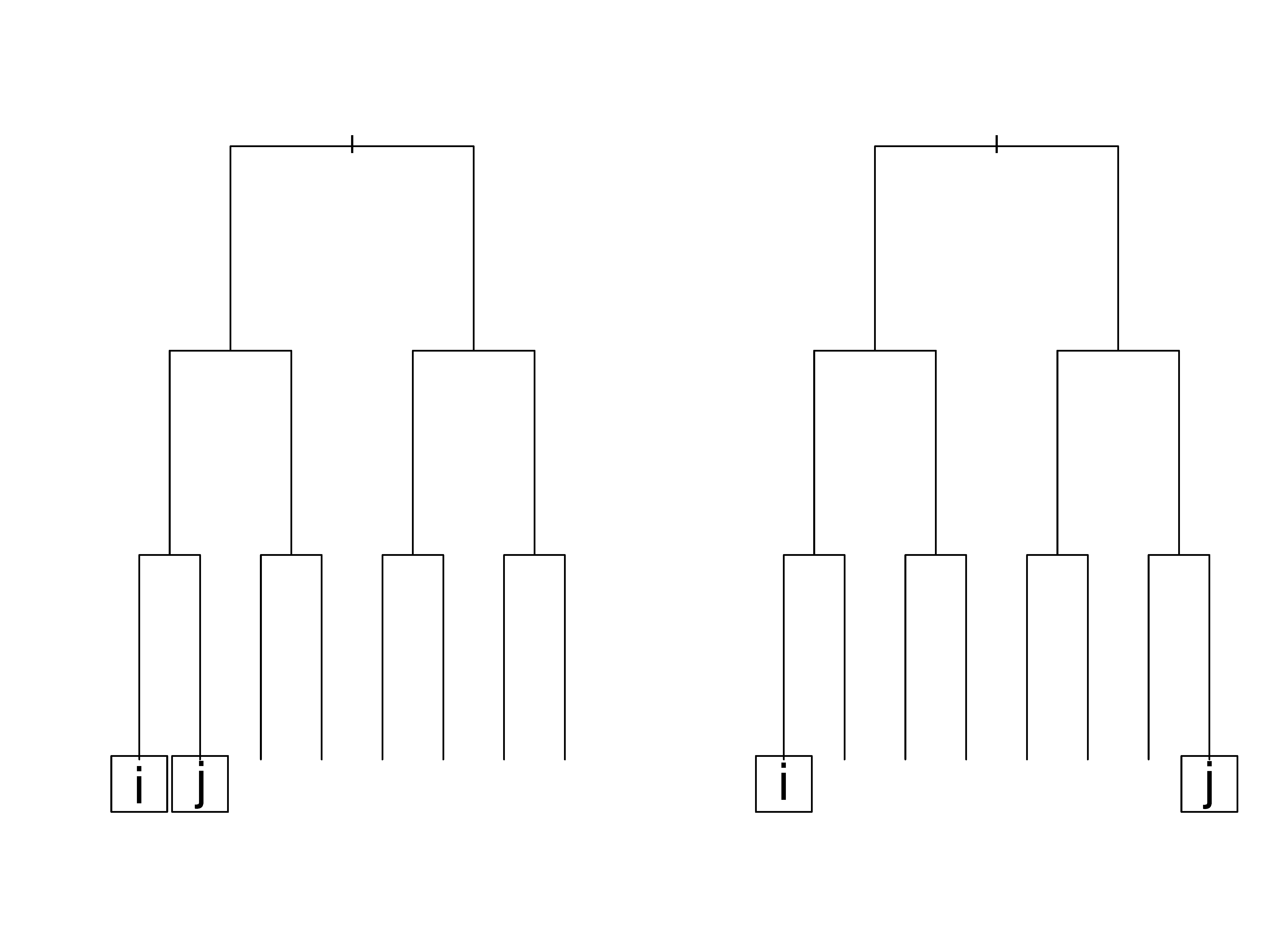
Simple illustration of RF distance
As a simple illustration, consider the tree \(T\) in Figure 1. In the first case (left figure), there is one split between both \(i\)’s and \(j\)’s terminal node and their lowest common node; therefore, \(S({\bf Z}_i,{\bf Z}_j,T)=2\) because it is the sum of splits to each terminal node. Also \(R({\bf Z}_i,{\bf Z}_j,T)=3+3=6\), because again, it is the sum for both nodes. The resulting distance measure for this particular tree between observations \(i\) and \(j\) is \(2/6\). Relatively speaking, we can think of the first case (left figure) being the one where \(i\) and \(j\) are considered to be much more similar to each other than in case two (right figure) where the lowest common node is the root node itself. In this latter case, \(D({\bf Z}_i,{\bf Z}_j,T)=R({\bf Z}_i,{\bf Z}_j,T) =6\) and the distance is one. From this we can see how the new measure can discern between the two cases above while the traditional proximity measure would have assigned both cases a value of zero since in neither case are observations \(i\) and \(j\) in the same terminal node.
Illustrating RF distance on the Iris data
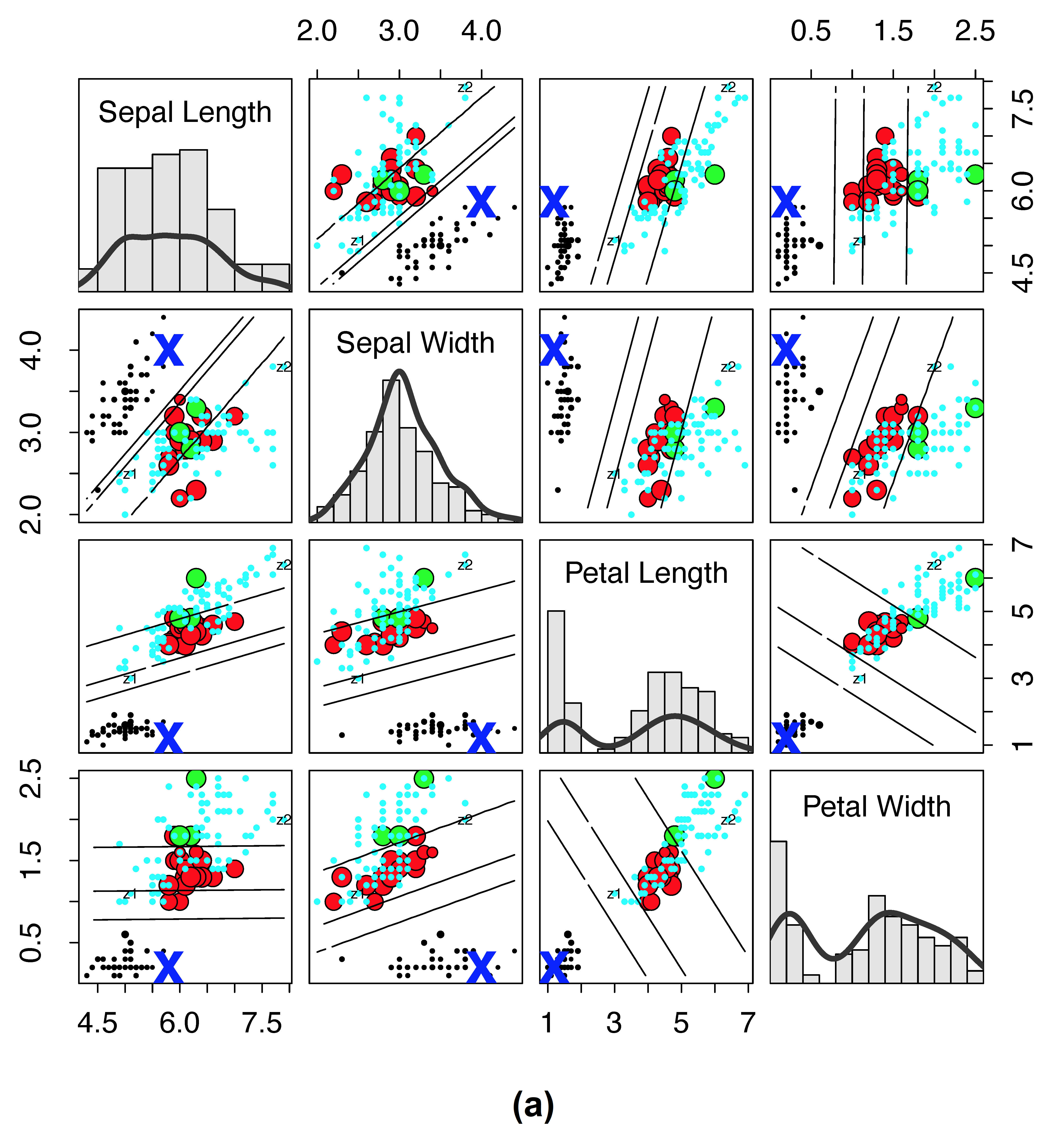
As another example, consider Figure 2, which plots RF proximity versus the new RF distance for the Iris data. Here we have selected a reference point denoted by “X” to observe how distance and proximity differ. The size of points have been scaled by their proximity (or their distance) to “X” so that a small size reflects closeness. If proximity is zero or distance is one, then a point is color coded by cyan (for visibility these cyan points are depicted using small circles).
Figure 2
 \(\quad\)
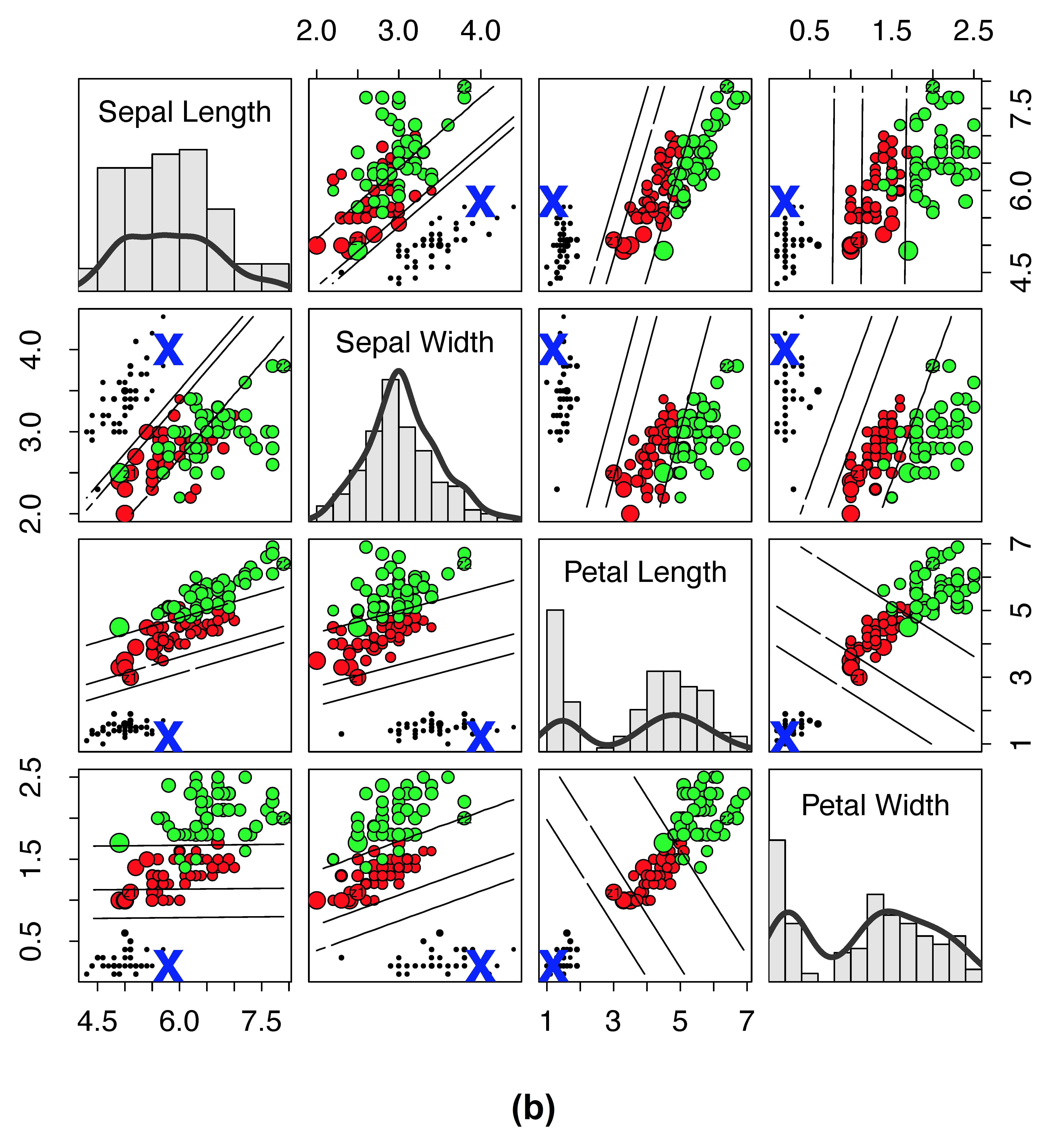
Traditional RF proximity versus new RF distance on Iris data. (a) Iris data where size of points are scaled by \(1-\log(1-\text{proximity})\) to the reference point “X” (lines depict LDA decision boundary between clusters). Points are color coded by cluster except if the proximity is zero, then it is cyan (for visibility, cyan points are always depicted using small points). (b) Same as (a), except that values are calculated using the new RF distance and size of points are scaled by \(1-\log(\text{distance})\). There are no cyan points because there are no points with distance of one to the reference point “X.”
Notice for proximity (subpanel (a)) that many points are cyan, meaning these points are equidistant and far from the reference point of interest. This is the result of the very stringent cutoff that RF proximity has for counting the proximity between two points.
In contrast, distance (subpanel (b)) can result in the value of one only under the extreme case that data points diverge after the root node split. The new distance allows for even small differences in the relatedness between points to be observed. Thus we see no cyan points in subpanel (b). Another important point is that distance appears to be smooth throughout much of the region and it is possible to observe where observations from different clusters are more similar to the point of interest, and where the points become different irrespective of the their true cluster membership.
Sidification
Algorithm 2 provides a detailed description of the sidification procedure used in Line 2 of the sidClustering procedure. Lines 2 and 3 of Algorithm 2 Sidification translate continuous features to be positive with the same maximum value and then reorders them by their range. This improves separation of distance between certain types of clusters. Lines 4-8 are the staggering process which results in the main SID main features \(({\bf Y}_i)_{i=1}^n\) (see Line 9). Lines 10-16 form pairwise interactions of main SID features resulting in the SID interaction features \(({\bf Z}_i)_{i=1}^n\) described in Line 17. The algorithm returns the sidified data \(\mathscr{L}^S=({\bf Z}_i,{\bf Y}_i)_{i=1}^n\) in Line 19.
Algorithm 2 Sidification
1: procedure Sidification \(({\bf X}_i)_{i=1}^n\),\(\delta=1\)
2: \(\quad\) Translate each continuous feature so that they are positive and all have the same maximum value (note that the minimum value can differ over variables)
3: \(\quad\) Order the variables in terms of their range with variables with largest range appearing first. This applies only to continuous variables (factors are placed randomly at the end)
4: \(\quad\) Convert any categorical variable with more than two categories to a set of zero-one dummy variables with one for each category
5: \(\quad\) Add \(\delta\) to the first variable
6: \(\quad\) for number of input variables, excluding the first do
7: \(\quad\quad\) Add \(\delta\) plus the maximum of the previous input variable to the current variable
8: \(\quad\) end for
9: \(\quad\) \(({\bf X}_i)_{i=1}^n\) have now been staggered
10: \(\quad\) for all pairs of main SID features (from Line 9) do
11: \(\quad\quad\) if a pair consists of two dummy variables then
12: \(\quad\quad\quad\) Interaction is a four level factor for each dummy variable combination
13: \(\quad\quad\) else
14: \(\quad\quad\quad\) Create interaction variable by multiplying them
15: \(\quad\quad\) end if
16: \(\quad\) end for
17: \(\quad\) This yields \(({\bf Z}_i)_{i=1}^n\) the SID interaction features
18: end procedure
19: return \(\mathscr{L}^S=({\bf Z}_i,{\bf Y}_i)_{i=1}^n\) the sidified data
Performance metrics
Performance metrics are implemented by the utility sid.perf.metric. The utitility provides performance assessements based on Gini and entropy, which are related to mutual information proposed by [9]. These measures function as weighted averages of impurity in the predicted clusters. Weights are determined by cluster size which then takes into count the possibility of gaming the measure by forming small clusters. Smaller clusters have a higher chance of being pure by random chance but their contribution to the score is reduced to compensate. The idea is that we want clusters that are both as large and pure as possible in order to obtain the best possible score.
The entropy and Gini measures of performance are defined as follows: \[ \rho_{\textrm E}=\sum_{i=1}^k \frac{n_i}{n} \sum_{j=1}^{k_t} -\frac{L_{ij}}{n_i}\log_2\left(\frac{L_{ij}}{n_i}\right), \hskip25pt \rho_{\textrm G}=\sum_{i=1}^k \frac{n_i}{n} \sum_{j=1}^{k_t} \frac{L_{ij}}{n_i}\left(1-\frac{L_{ij}}{n_i}\right), \] where: \[ \begin{array}{lcl} n &=& \text{total number of cases}\\ n_i &=& \text{number of cases in cluster $i$}\\ k_t &=& \text{number of clusters targeted by clustering algorithm}\\ k &=& \text{true number of clusters}\\ L_{ij} &=& \text{number of cases when predicted cluster label is $j$ when true label is $i$}. \end{array} \] A normalized measure is also provided by normalizing the metrics to a range of 0 to 1 by dividing by the maximum value which occurs under uniform guessing. A lower score indicates better overall clustering. Also, users may consider squaring the normalized measures as these retain the 0 to 1 range and add a middle point of comparison where a score of 0.5 corresponds with 50% correct clustering. It should also be noted that these are measures of purity which are robust to label switching since our goal is to determine ability to cluster similar observations.
Illustration
library(randomForestSRC)
o <- sidClustering(iris[, -5], k = 3)
print(table(iris[, 5], o$cl))

>
>               1  2  3
>   setosa     50  0  0
>   versicolor  4 44  2
>   virginica   0 14 36
The table at the bottom is the confusion matrix obtained from the clusters found by unsupervised analysis using sidClustering (notice the analysis is unsupervised since we have removed the Iris classification label, “Species,” which is the fifth column of the data). To assess clustering performance of sidClustering, we now compare the clusters found by the method compared to the actual true class labels. Performance is assessed using the sid.perf.metric utility function, which is listed below.
print(sid.perf.metric(iris$Species, o$clustering))

> $result
>         1
> 0.6109346
>
> $measure
> [1] "entropy"
>
> $normalized_measure
>         1
> 0.3854568
In the above output, the $result is the entropy measure, \(\rho_E\); the $normalize_measure is normalized \(\rho_E\).
Cite this vignette as
H. Ishwaran, A. Mantero, M. Lu, and U. B. Kogalur. 2021. “randomForestSRC: sidClustering vignette.” http://randomforestsrc.org/articles/sidClustering.html.
@misc{HemantsidClustering,
    author = "Hemant Ishwaran and Alejandro Mantero and Min Lu and Udaya B. Kogalur",
    title = {{randomForestSRC}: {sidClustering} vignette},
    year = {2021},
    url = {http://randomforestsrc.org/articles/sidClustering.html},
    howpublished = "\url{http://randomforestsrc.org/articles/sidClustering.html}",
    note = "[accessed date]"
}