Random Survival Forests
Hemant Ishwaran
Michael S. Lauer
Eugene H. Blackstone
Min Lu
Udaya B.
Kogalur
2026-01-30
survival.Rmd
Introduction
Early applications of random forests (RF) focused on regression and classification problems. Random survival forests [1] (RSF) was introduced to extend RF to the setting of right-censored survival data. Implementation of RSF follows the same general principles as RF: (a) Survival trees are grown using bootstrapped data; (b) Random feature selection is used when splitting tree nodes; (c) Trees are generally grown deeply, and (d) The survival forest ensemble is calculated by averaging terminal node statistics (TNS).
The presence of censoring is a unique feature of survival data that complicates certain aspects of implementing RSF compared to RF for regression and classification. In right-censored survival data, the observed data is where is time and is the censoring indicator. The observed time is defined as the minimum of the true (potentially unobserved) survival event time and the true (potentially unobserved) censoring time ; thus and the actual event time might not be observed. The censoring indicator is defined as . When , an event has occurred (i.e., death has occurred) and we observe the true event time, . Otherwise when , the observation is censored and we only observe the censoring time : thus we know that the subject has survived to time , but not when the subject actually dies.
Hereafter we denote the data by where is the feature vector (covariate) for individual and and are the observed time and censoring indicators for . RSF trees just like RF trees are grown using resampling (for example by using the bootstrap; the default is to use .632 sampling without replacement). However for notational simplicity, we will sometimes ignore this distinction.
RSF splitting rules
The true event time being subject to censoring must be dealt with when growing a RSF tree. In particular, the splitting rule for growing the tree must specifically account for censoring. Thus, the goal is to split the tree node into left and right daughters with dissimilar event history (survival) behavior.
Log-rank splitting
The default splitting rule used by the package is the log-rank test
statistic and is specified by splitrule="logrank". The
log-rank test has traditionally been used for two-sample testing with
survival data, but it can be used for survival splitting as a means for
maximizing between-node survival differences [2–6].
To explain log-rank splitting, consider a specific tree node to be split. Without loss of generality let us assume this is the root node (top of the tree). For simplicity assume the data is not bootstrapped, thus the root node data is . Let denote a specific variable (i.e., one of the coordinates of the feature vector). A proposed split using is of the form and (for simplicity we assume is nominal) and splits the node into left and right daughters, and , respectively. Let be the distinct death times and let and equal the number of deaths and individuals at risk at time in daughter nodes . At risk means the number of individuals in a daughter who are alive at time , or who have an event (death) at time : Define The log-rank split-statistic value for the split is The value is a measure of node separation. The larger the value, the greater the survival difference between and , and the better the split is. The best split is determined by finding the feature and split-value such that for all and .
Log-rank score splitting
The package also implements splitting using the log-rank score test
[7]. This is specified by the option
splitrule="logrankscore". To describe this rule, assume the
variable
has been ordered so that
where for simplicity
we assume there are
unique values for
(no ties). Now compute the ``ranks’’ for each survival time
,
where
.
The log-rank score test is defined as
where
and
are the sample mean and sample variance of
and
where
is the sample size of the left daughter node. Log-rank score splitting
defines the measure of node separation by
.
Maximizing this value over
and
yields the best split.
Randomized splitting
All models in the package including RSF allow the use of randomized
splitting specified by the option nsplit. Rather than
splitting the node by considering all possible split-values for a
variable, instead a fixed number of randomly selected split-points
are chosen [1, 8, 9]. For example, the
best randomized split using log-rank splitting is the maximal value of
For each variable
,
this reduces
split-statistic evaluations (worst case scenario) to
evaluations. Not only does randomized splitting greatly reduce
computations, it also mitigates the well known tree bias of favoring
splits on variables with a large number of split-points, such as
continuous variables or factors with a large number of categorical
labels [10]. Related work includes [11] who investigated extremely randomized
trees. Here a single random split-point is chosen for each variable
(i.e.,
).
Traditional deterministic splitting (all split values considered) is
specified by nsplit = 0.
Terminal node statistics (TNS)
RSF estimates the survival function, , and the cumulative hazard function (CHF), Below we describe how these two quantities are estimated using a survival tree.
In-bag (IB) estimator
Once the survival tree is grown, the ends of the tree are called the terminal nodes. The survival tree predictor is defined in terms of the predictor within each terminal nodel. Let be a terminal node of the tree and let be the unique death times in and let and equal the number of deaths and individuals at risk at time . The CHF and survival functions for are estimated using the bootstrapped Nelson-Aalen and Kaplan-Meier estimators The survival tree predictor is defined by assigning all cases within the same CHF and survival estimate. This is because the purpose of the survival tree is to partition the data into homogeneous groups (i.e., terminal nodes) of individuals with similar survival behavior. To estimate and for a given feature , drop down the tree. Because of the binary nature of a tree, will fall into a unique terminal node . The CHF and survival estimator for equals the Nelson-Aalen and Kaplan-Meier estimator for ’s terminal node: Note that we use the notation IB because the above estimators are based on the training data, which is the IB data.
Ensemble CHF and Survival Function
The ensemble CHF and survival function are determined by averaging the tree estimator. Let and be the IB CHF and survival estimator for the th survival tree. The IB ensemble estimators are Let record trees where case is OOB. The OOB ensemble estimators for individual are An important distinction between the two sets of estimators is that OOB estimators are used for inference on the training data and for estimating prediction error. In-bag estimators on the other hand are used for prediction and can be used for any feature .
Why are two estimates provided?
Why does RSF estimate both the CHF and the survival function? Classically, we know the two are related by The problem is that even if it were true that for every tree , the above identity will not hold for the ensemble. Let and denote the ensemble survival and CHF and let denote ensemble expectation (i.e., and ). Then by Jensen’s inequality for convex functions, In other words, of the survival ensemble does not necessarily equal the ensemble of of the tree survival function. The inequality above also shows that taking of the ensemble survival will generally be smaller than the true ensemble CHF. This is why RSF provides the two values separately.
Prediction error
Prediction error for survival models is measured by , where C is Harrell’s concordance index [12]. Prediction error is between 0 and 1, and measures how well the predictor correctly ranks two random individuals in terms of survival. Unlike other measures of survival performance, Harrell’s C-index does not depend on choosing a fixed time for evaluation of the model and specifically takes into account censoring of individuals. The method is a popular means for assessing prediction performance in survival settings since it is easy to understand and interpret.
Mortality (the predicted value used by RSF)
To compute the concordance index we must define what constitutes a worse predicted outcome. For survival models this is defined by the concept of mortality which is the predicted value used by RSF. Let denote the entire set of unique event times for the learning data. The IB ensemble mortality for a feature is defined as This estimates the number of deaths expected if all cases were similar to . OOB ensemble mortality which is used for the C-index calculation is defined by Individual is said to have a worse outcome than individual if
The mortality value [1] represents estimated risk for each individual calibrated to the scale of the number of events. Thus as a specific example, if has a mortality value of 100, then if all individuals had the same covariate as , which is , we would expect an average of 100 events.
C-index calculation
The C-index is calculated using the following steps:
Form all possible pairs of observations over all the data.
Omit those pairs where the shorter event time is censored. Also, omit pairs if unless or or . The last restriction only allows ties in event times if at least one of the observations is a death. Let the resulting pairs be denoted by . Let permissible .
If , count 1 for each in which the shorter time had the worse predicted outcome.
If , count 0.5 for each in which .
If , count 1 for each in which .
If , count 0.5 for each in which .
Let concordance denote the resulting count over all permissible pairs. Define the concordance index C as
- The error rate is $\tt PE=1−C$. Note that $0≤\tt PE≤1$ and that $\tt PE=0.5$ corresponds to a procedure doing no better than random guessing, whereas $\tt PE=0$ indicates perfect prediction.
Brier score
The Brier score, , is another popular measure used to assess prediction peformance. Let be some estimator of the survival function. To estimate the prediction performance of , let be a prechosen estimator of the censoring survival function, . The Brier score for can be estimated by using inverse probability of censoring weights (IPCW) using the method of [13] The integrated Brier score at time is defined as which can be estimated by substituting for . Lower values for the Brier score indicate better prediction performance. Using the Brier score we can calculate the continuous rank probability score (CRPS), defined as the integrated Brier score divided by time.
Illustration
To illustrate, we use the survival data from [14] consisting of 2231 adult patients with systolic heart failure. All patients underwent cardiopulmonary stress testing. During a mean follow-up of 5 years (maximum for survivors, 11 years), 742 patients died. The outcome is all-cause mortality and a total of covariates were measured for each patient including demographic, cardiac and noncardiac comorbidity, and stress testing information.
library(randomForestSRC)
data(peakVO2, package = "randomForestSRC")
dta <- peakVO2
obj <- rfsrc(Surv(ttodead,died)~., dta,
             ntree = 1000, nodesize = 5, nsplit = 50, importance = TRUE)
print(obj)

>  1                          Sample size: 2231
>  2                     Number of deaths: 726
>  3                      Number of trees: 1000
>  4            Forest terminal node size: 5
>  5        Average no. of terminal nodes: 259.368
>  6 No. of variables tried at each split: 7
>  7               Total no. of variables: 39
>  8        Resampling used to grow trees: swor
>  9     Resample size used to grow trees: 1410
> 10                             Analysis: RSF
> 11                               Family: surv
> 12                       Splitting rule: logrank *random*
> 13        Number of random split points: 50
> 14                           (OOB) CRPS: 1.52830075
> 15              (OOB) standardized CRPS: 0.15497275
> 16    (OOB) Requested performance error: 0.29830498
From the above code, obj$survival
obj$survival.oob and obj$chf
obj$chf.oob contain the IB and OOB survival functions and
CHFs respectively. All these four objects have a dimension of
,
where
is number of patients and
is number of unique time points from the inputted argument
ntime, and all the unique death times are ordered and
stored in obj$time.interest. The one-dimensional predicted
values are stored in obj$predicted and
obj$predicted.oob, which are IB and OOB mortality. The
continuous rank probability score (CRPS) is shown in line 14 which is
defined as the integrated Brier score divided by time. The Brier score
is calculated using inverse probability of censoring weights (IPCW)
using the method of Gerds et al. (2006) [13]. The error rate is stored in
obj$err.rate which is calculated using the C-calculation as
described above and is
shown in line 15. For the printout, line 2 displays the number of
deaths; line 3 and 4 displays the number of trees and the size of
terminal node, which are specified by the input argument
ntree and nodesize. Line 5 displays the number
of terminal nodes per tree averaged across the forest and line 6
reflects the input argument mtry, which is the number of
variables randomly selected as candidates for splitting a node; line 8
displays the type of bootstrap, where swor refers to
sampling without replacement and swr refers to sampling
with replacement; line 9 displays the sample size for line 8 where for
swor, the number equals to about 63.2% observations, which
matches the ratio of the original data in sampling with replacement;
line 10 and 11 show the type of forest where RSF and
surv refer to family survival; line 12
displays splitting rule
which matches the inputted argument splitrule and line 13
shows the number of random splits to consider for each candidate
splitting variable which matches the inputted argument
nsplit.
The following illustrates how to get the C-index directly from a RSF analysis using the built in function get.cindex.
Plot the estimated survival functions
Figure 1 displays the (in-bag) predicted
survival functions for two hypothetical individuals, where all
features of the two individuals are set to the median level except for
the variable peak
VO.
These two individuals were defined in the following code in
newdata, whose predictions were stored in
y.pred which was plotted in the next block of code. For one
of the individuals this is set at the 25th quantile for peak
VO
(peak
VO
mL/kg per min) and shown using a solid black line. For the other
individual this was set to the 75th quantile (peak
VO
mL/kg per min) and shown using a dashed red line.
newdata <- data.frame(lapply(1:ncol(obj$xvar),function(i){median(obj$xvar[,i])}))
colnames(newdata) <- obj$xvar.names
newdata1 <- newdata2 <- newdata
newdata1[,which(obj$xvar.names == "peak_vo2")] <- quantile(obj$xvar$peak_vo2, 0.25)
newdata2[,which(obj$xvar.names == "peak_vo2")] <- quantile(obj$xvar$peak_vo2, 0.75)
newdata <- rbind(newdata1,newdata2)
y.pred <- predict(obj,newdata = rbind(newdata,obj$xvar)[1:2,])
pdf("survival.pdf", width = 10, height = 8)
par(cex.axis = 2.0, cex.lab = 2.0, cex.main = 2.0, mar = c(6.0,6,1,1), mgp = c(4, 1, 0))
plot(round(y.pred$time.interest,2),y.pred$survival[1,], type="l", xlab="Time (Year)",
     ylab="Survival", col=1, lty=1, lwd=2)
lines(round(y.pred$time.interest,2), y.pred$survival[2,], col=2, lty=2, lwd=2)
legend("topright", legend=c("Peak VO2=12.8","Peak VO2=19.3"), col=c(1:2), lty=1:2, cex=2, lwd=2)
dev.off() 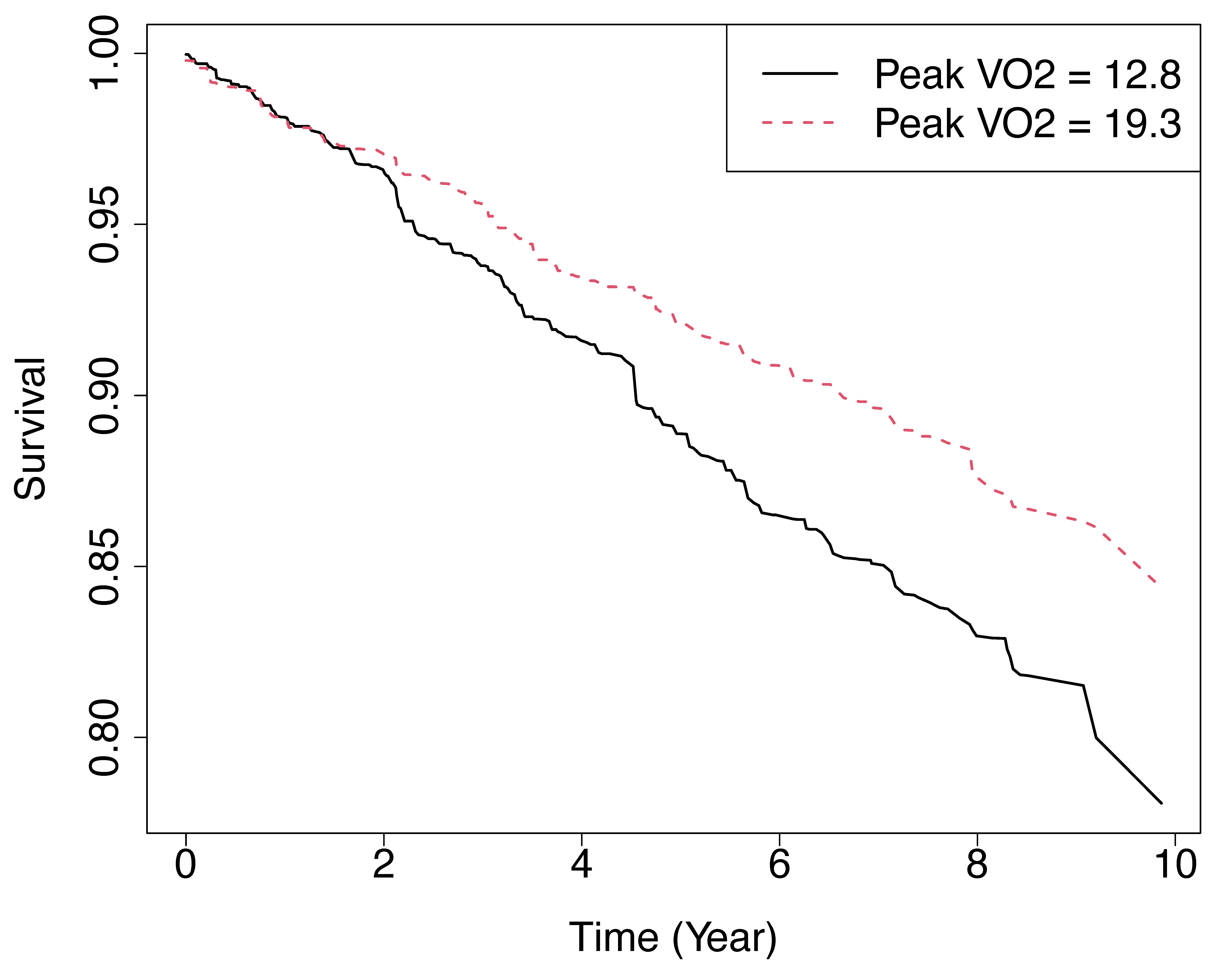
Figure 1
Predicted survival functions for two hypothetical individuals from RSF analysis of systolic heart failure data. Solid black line represents individual with peak VO mL/kg per min. Red dash line represents individual with peak VO mL/kg per min. All other variables for both individuals are set to the median value.
Plot the Brier Score and Calculate the CRPS
Figure 2 displays the Brier
for the RSF analysis of the heart failure data given above. These values
are obtained by using the function get.brier.survival. In
this function, two methods are available for estimating the censoring
distribution used for the IPCW. The first method uses the Kaplan-Meier
censoring distribution estimator and the second using a RSF censoring
distribution estimator. The results are given below:
## obtain Brier score using KM and RSF censoring distribution estimators
bs.km <- get.brier.survival(obj, cens.mode = "km")$brier.score
bs.rsf <- get.brier.survival(obj, cens.mode = "rfsrc")$brier.score

## plot the brier score
plot(bs.km, type = "s", col = 2)
lines(bs.rsf, type ="s", col = 4)
legend("bottomright", legend = c("cens.model = km", "cens.model = rfsrc"), fill = c(2,4))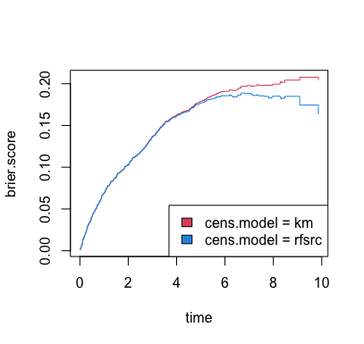
Figure 2
The Brier score can be used to obtain other information, such as the
CRPS. The get.brier.survival function actually returns this
value, but below we show how to extract CRPS for ever time point
directly from the previously estimated Brier score.
## here's how to calculate the CRPS for every time point
trapz <- randomForestSRC:::trapz
time <- obj$time.interest
crps.km <- sapply(1:length(time), function(j) {
  trapz(time[1:j], bs.km[1:j, 2] / diff(range(time[1:j])))
})
crps.rsf <- sapply(1:length(time), function(j) {
  trapz(time[1:j], bs.rsf[1:j, 2] / diff(range(time[1:j])))
})

## plot CRPS as function of time
plot(time, crps.km, ylab = "CRPS", type = "s", col = 2)
lines(time, crps.rsf, type ="s", col = 4)
legend("bottomright", legend=c("cens.model = km", "cens.model = rfsrc"), fill=c(2,4))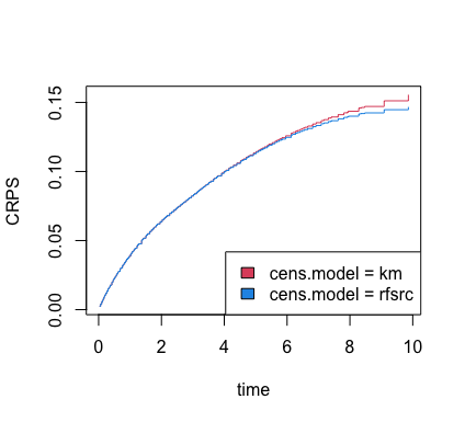
Variable Importance
RSF provides a fully nonparametric measure of variable importance (VIMP). The most common measure is Breiman-Cutler VIMP [15] and is called permutation importance. VIMP calculated using permutation importance adopts a prediction based approach by measuring prediction error attributable to the variable. A clever feature is that rather than using cross-validation, which can be computationally expensive, permutation importance makes use of OOB estimation. Specifically, to calculate the VIMP for a variable , we randomly permute the OOB values of in a tree (the remaining coordinates of are not altered). The perturbed OOB data is dropped down the tree and the OOB error for the resulting tree predictor determined. The amount by which this new error exceeds the original OOB error for the tree equals the tree importance for . Averaging over trees yields permutation importance for .
Large positive VIMP indicates high predictive ability while zero or negative values identify noise variables. Subsampling [16] can be used to estimate the standard error and to approximate the confidence intervals for VIMP. Figure 3 displays delete- jackknife 99% asymptotic normal confidence intervals for the variables from the systolic heart failure RSF analysis. Prediction error was calculated using the C-index.
  jk.obj <- subsample(obj)
  pdf("VIMPsur.pdf", width = 15, height = 20)
  par(oma = c(0.5, 10, 0.5, 0.5))
  par(cex.axis = 2.0, cex.lab = 2.0, cex.main = 2.0, mar = c(6.0,17,1,1), mgp = c(4, 1, 0))
  plot(jk.obj, xlab = "Variable Importance (x 100)", cex = 1.2)
  dev.off()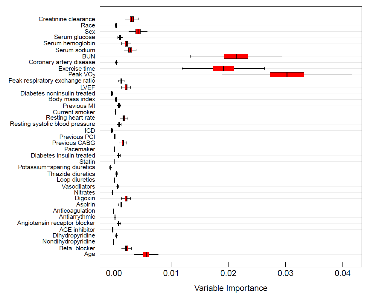
Figure 3
Delete-d jackknife 99% asymptotic normal confidence intervals of VIMP from RSF analysis of systolic heart failure data. Prediction error is defined using Harrell’s concordance index.
Cite this vignette as
H. Ishwaran, M. S.
Lauer, E. H. Blackstone, M. Lu, and U. B. Kogalur. 2021.
“randomForestSRC: random survival forests vignette.” http://randomforestsrc.org/articles/survival.html.
@misc{HemantRandomS,
    author = "Hemant Ishwaran and Michael S. Lauer and Eugene H. Blackstone and Min Lu
               and Udaya B. Kogalur",
    title = {{randomForestSRC}: random survival forests vignette},
    year = {2021},
    url = {http://randomforestsrc.org/articles/survival.html},
    howpublished = "\url{http://randomforestsrc.org/articles/survival.html}",
    note = "[accessed date]"
}