
Introduction
Partial dependence plots, or sometimes just referred to as partial plots, were introduced by [1] as a visualization tool for exploring the relationship between the features and the outcome in a supervised learning problem. Let \(F({\bf x})\) be the target function in the supervised problem where \({\bf x}=(x_{1},\ldots,x_{p})\) is the \(p\)-dimensional feature. Let \({\bf x}_s\) denote \({\bf x}\) restricted to coordinate indices \(s\subset\{1,\ldots,p\}\). Likewise using the notation \(\mathbin{\smallsetminus} s=\{1,\ldots,p\}\smallsetminus s\) to denote the complement of \(s\), let \({\bf x}_{\mathbin{\smallsetminus} s}\) denote the coordinates of \({\bf x}\) with indices not in \(s\).
Definition 1: The (marginal) partial dependence function is \[ \bar{F}_{s}({\bf x}_s) = \int F({\bf x}_s, {\bf x}_{\mathbin{\smallsetminus} s})p_{\mathbin{\smallsetminus} s}({\bf x}_{\mathbin{\smallsetminus} s})\,d{\bf x}_{\mathbin{\smallsetminus} s} \] where \(p_{\mathbin{\smallsetminus} s}({\bf x}_{\mathbin{\smallsetminus} s})\) is the marginal probability density of \({\bf x}_{\mathbin{\smallsetminus} s}\), \(p_{\mathbin{\smallsetminus} s}({\bf x}_{\mathbin{\smallsetminus} s}) = \int p({\bf x})\,d{\bf x}_s\).
Simply put, the partial dependence function for \({\bf x}_s\) is obtained by integrating out the remaining variables. Of course in practice we do not know the feature distribution. And in the supervised learning problem we also do not know \(F\) but estimate it using our supervised method. For example, in random forests we estimate \(F\) by using an ensemble of trees. Call this estimator \(\hat{F}\). Let \({\bf X}_1,\ldots,{\bf X}_n\) denote the features from the learning data, then the estimated partial dependence function is \[ \hat{\bar{F}}({\bf x}_s) = \frac{1}{n}\sum_{i=1}^n \hat{F}({\bf x}_s,{\bf X}_{i,\mathbin{\smallsetminus} s}). \] Therefore, the coordinates of \({\bf X}_i\) corresponding to \(s\) are replaced by \({\bf x}_s\) yielding a new feature \(({\bf x}_s,{\bf X}_{i,\mathbin{\smallsetminus} s})\) for \(i=1,\ldots,n\). Evaluation of this with respect to \(\hat{F}\) and then averaging yields the estimated partial dependence function.
plot.variable
The package provides a convenient function plot.variable
for creating partial plots. By default the function produces marginal
(unadjusted) figures and simply plots the predicted values \(F({\bf X}_i)\). In order to obtain partial
plots, we need to set the option partial=TRUE.
Below is an illustration using the airquality() data. As
this is a regression problem, the target function is \(F({\bf x})=\mathbb{E}(Y|{\bf X}={\bf x})\),
the conditional mean of the outcome \(Y\) given \({\bf
X}={\bf x}\). In this example, the partial plot for the variable
“Wind” is provided.
library(randomForestSRC)
# New York air quality measurements
airq.obj <- rfsrc(Ozone ~ ., data = airquality)
plot.variable(airq.obj, xvar.names = "Wind", partial = TRUE)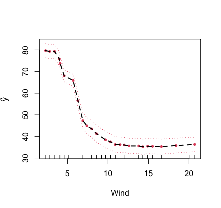
The plot.variable function can also be used for
multivariate forests. To do so, we need to specify the outcome of
interest, which could either be real valued (corresponding to
regression) or a factor (corresponding to classification).
The following example converts some of the features from the
mtcars() data to factors to illustrate a mixed multivariate
forest application. There are three outcomes, “carb”, “mpg” and “cyl”.
The outcome “mpg” is continuous, while the two other outcomes are
factors. To specify the outcome to be used for the partial plot, we use
the option m.target. In our example we set
m.target='cyl' which is a factor and correspond to a
classification analysis. For classification, the function of interest
\(F({\bf x})\) is the conditional
probability \(\mathbb{P}\{Y=C_j|{\bf X}={\bf
x}\}\) where \(C_j\) is the
\(j\)th class label. By default, the
first class label \(C_1\) is used,
however the option target can be used to change this. The
latter can either be an integer (specifying the index of the level of
the factor to be used) or a character vector giving the actual class
label value.
## use mtcars, but make some factors
mtcars2 <- mtcars
mtcars2$carb <- factor(mtcars2$carb)
mtcars2$cyl <- factor(mtcars2$cyl)

## run multivariate forests
mtcars.mix <- rfsrc(Multivar(carb, mpg, cyl) ~ ., data = mtcars2)
levels(mtcars2$cyl)
> [1] "4" "6" "8"

## there are three class labels for the outcome cylinder
## partial plot for displacement for class label "4" of cylinder
plot.variable(mtcars.mix, m.target = "cyl", target = "4",
       xvar.names = "disp", partial = TRUE)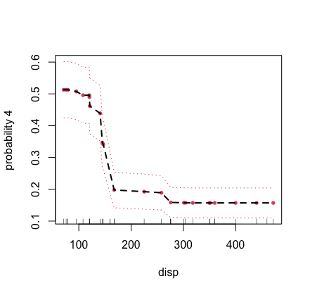
partial
The function plot.variable is just a convenient
interface to the more powerful function partial. The latter
is much faster and can be customized for sophisticated partial plot
analyses.
Here’s the previous example for the airquality data
using a direct call to partial. Notice that we use the
helper function get.partial.plot.data, which is a useful
utility for parsing the partial plot data returned from
partial.
## first run the forest
airq.obj <- rfsrc(Ozone ~ ., data = airquality)

## partial effect for wind
partial.obj <- partial(airq.obj,
                 partial.xvar = "Wind",
                 partial.values = airq.obj$xvar$Wind)

## helper function for extracting the partial effects
pdta <- get.partial.plot.data(partial.obj)

## plot partial values
plot(pdta$x, pdta$yhat, type = "b", pch = 16,
     xlab = "wind", ylab = "partial effect of wind")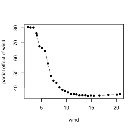
Here’s a more complicated example showing how to calculate a
bivariate partial plot. We use the airquality data for a
bivariate partial plot of variables “Wind” and “Temp’’.
## first run the forest
airq.obj <- rfsrc(Ozone ~ ., data = airquality)

## specify wind and temperature values of interest
wind <- sort(unique(airq.obj$xvar$Wind))
temp <- sort(unique(airq.obj$xvar$Temp))

## partial effect for wind, for a given temp
pdta <- do.call(rbind, lapply(temp, function(x2) {
       o <- partial(airq.obj,
             partial.xvar = "Wind", partial.xvar2 = "Temp",
             partial.values = wind, partial.values2 = x2)
       cbind(wind, x2, get.partial.plot.data(o)$yhat)
     }))
pdta <- data.frame(pdta)
colnames(pdta) <- c("wind", "temp", "effectSize")

## coplot of partial effect of wind and temp
coplot(effectSize ~ wind|temp, pdta, pch = 16, overlap = 0)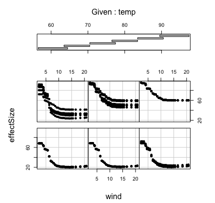
Our final example considers a survival setting. This is more complicated because with survival there are always many choices for the target \(F\). For example, we might be interested in survival, in which case the estimated partial effects for survival for a variable \(x_s\) is \[ \hat{\bar{F}}(t|x_s) = \frac{1}{n}\sum_{i=1}^n \hat{S}(t|x_s,{\bf X}_{i,\mathbin{\smallsetminus} s}) \] where \(\hat{S}(t|{\bf x})\) is the forest estimated survival function at time \(t\) for feature \({\bf x}\). Notice that the partial effect is a function of \(x_s\) and time \(t\).
The following example uses the veteran() data for
illustration. We consider partial effects for mortality and
survival.
## run rsf on veteran data
data(veteran, package = "randomForestSRC")
v.obj <- rfsrc(Surv(time,status)~., veteran, nsplit = 10, ntree = 100)
## get partial effect of age on mortality
partial.obj <- partial(v.obj,
partial.type = "mort",
partial.xvar = "age",
partial.values = v.obj$xvar$age,
partial.time = v.obj$time.interest)
pdta <- get.partial.plot.data(partial.obj)
## plot partial effect of age on mortality
plot(lowess(pdta$x, pdta$yhat, f = 1/3),
type = "l", xlab = "age", ylab = "adjusted mortality")
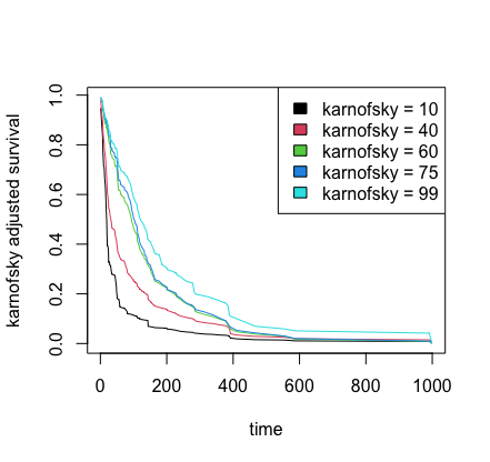
## partial effects of karnofsky score on survival
karno <- quantile(v.obj$xvar$karno)
partial.obj <- partial(v.obj,
partial.type = "surv",
partial.xvar = "karno",
partial.values = karno,
partial.time = v.obj$time.interest)
pdta <- get.partial.plot.data(partial.obj)
## plot partial effect of karnofsky on survival
matplot(pdta$partial.time, t(pdta$yhat), type = "l", lty = 1,
xlab = "time", ylab = "karnofsky adjusted survival")
legend("topright", legend = paste0("karnofsky = ", karno), fill = 1:5)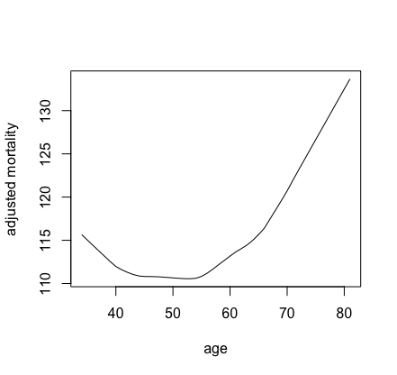
Cite this vignette as
H. Ishwaran, M. Lu, and
U. B. Kogalur. 2021. “randomForestSRC: partial plots vignette.” http://randomforestsrc.org/articles/partial.html.
@misc{HemantPartial,
    author = "Hemant Ishwaran and Min Lu and Udaya B. Kogalur",
    title = {{randomForestSRC}: partial plots vignette},
    year = {2021},
    url = {http://randomforestsrc.org/articles/partial.html},
    howpublished = "\url{http://randomforestsrc.org/articles/partial.html}",
    note = "[accessed date]"
}