Getting starting with the randomForestSRC R-package for random forest analysis of regression, classification, survival and more
Hemant Ishwaran
Min Lu
Udaya B.
Kogalur
getstarted.Rmd
Introduction
randomForestSRC is a CRAN
compliant R-package implementing Breiman random forests [1] in a variety of problems. The package uses
fast OpenMP parallel processing to construct forests for regression,
classification, survival analysis, competing risks, multivariate, unsupervised, quantile regression and class imbalanced
-classification.
The package is constantly being worked on and many new kinds of
applications, forests and tree constructions will be added to it in the
near future.
The package was developed by Hemant Ishwaran and Udaya Kogalur and is
the descendent of their original (and now retired) parent package
randomSurvivalForest for fitting survival data. Originally,
Breiman’s random forest (RF) was only available for regression and
classification. Random survival forests (RSF) [2] was
invented to extend RF to the setting of right-censored survival
data.
randomForestSRC has evolved over time so that it can now
construct many interesting forests for different applications. But then
what exactly is a forest — and what exactly is a random
forest?
Basically, a forest is an example of an ensemble, which is a special type of machine learning method that averages simple functions called base learners. The resulting averaged learner is called the ensemble. RF uses trees for the base-learner and builds on the ensemble concept by injecting randomization into the learning process — this is where the random in random forests comes from. Specifically, randomization is introduced in two forms. First, a randomly drawn bootstrap sample of the data is used to grow a tree (actually there is nothing special about the bootstrap, and other types of sampling are used). Second, during the grow stage at each node of the tree, a randomly selected subset of variables is chosen as candidates for splitting (this is called random feature selection). The purpose of this two-step randomization is to decorrelate trees, which reduces variance due to bagging [3]. Furthermore, RF trees are typically grown very deeply; in fact, Breiman’s original RF classifier called for growing a classification tree to purity (one observation per terminal node). The use of deep trees, a bias reduction technique, when combined with reduced variance due to averaging and randomization, enables RF to approximate rich classes of functions while maintaining low generalization error.
Why Does Random Forests Work? A More Technical Explanation
It might still seem like a mystery why averaging simple base-learners like trees leads to the excellent performance often reported with ensembles. Here we attempt to provide a more technical explanation for why this happens. This explanation applies to all kinds of ensembles and not just RF.
For simplicity, we consider the regression case. Let be a collection of learners where each learner is trained on the same learning data set $\mathscr{L}=\{({\bf X}_1,Y_1), \ldots, ({\bf X}_n,Y_n)\}$. The goal is to estimate the regression function $f({\bf X})$ which is the conditional mean of the scalar outcome conditional on the feature vector ${\bf X}\in{\mathscr X}$. It is assumed that each learner is trained separately from one another. Because the learners are trained on the same data they cannot be independent, however we will assume they share the same distribution. This assumption holds for RF.
Define the ensemble estimator as the averaged value of the learners $$ \hat{f}_{\text{ens}}({\bf x})=\frac{1}{B}\sum_{b=1}^B \varphi_b({\bf x}). $$ For example if the base-learners are trees, then is a tree ensemble like RF. Let $({\bf X},{\bf Y})$ be an independent test data point with the same distribution as the learning data. The generalization error for an estimator is $$ \text{Err}(\hat{f})= \mathbb{E}_\mathscr{L}\mathbb{E}_{{\bf X},Y}\Bigl[Y-\hat{f}({\bf X})\Bigr]^2. $$ Assuming a regression model $Y=f({\bf X})+\varepsilon$ where ${\bf X}\perp\varepsilon$ and , using a bias-variance decomposition, we have $$ \text{Err}(\hat{f}) = \sigma^2 + \mathbb{E}_{\bf X}\left\{\text{Bias}\{\hat{f}\,|\,{\bf X}\}^2 + \text{Var}\{\hat{f}\,|\,{\bf X}\}\right\} $$ where the two terms on the right are the conditional bias and conditional variance for . Using this notation, we can establish the following result [4].
Theorem
If are identically distributed learners constructed from , then $$ \text{Err}(\hat{f}_{\text{ens}}) = \sigma^2 + \mathbb{E}_{\bf X}\left\{\text{Bias}\{\varphi\,|\,{\bf X}\}^2 + \frac{1}{B}\text{Var}\{\varphi\,|\,{\bf X}\} + \left(1-\frac{1}{B}\right)\overline{\text{Cov}}({\bf X}) \right\} $$ where $\overline{\text{Cov}}({\bf X}) = {\text{Cov}}(\varphi_b,\varphi_{b'}|{\bf X})$.
To understand the above Theorem, keep in mind that the number of learners, , is at our discretion and can be selected as large as we want (of course in practice this decision will be affected by computational cost, but let’s not worry about that for now). Therefore with a large enough collection of learners we can expect the generalization error to closely approximate the limiting value $$ \lim_{B\rightarrow\infty} \text{Err}(\hat{f}_{\text{ens}}) = \sigma^2 + \mathbb{E}_{\bf X}\left\{\text{Bias}\{\varphi|\,{\bf X}\}^2 + \overline{\text{Cov}}({\bf X}) \right\}. $$ Notice that the variance has completely disappeared! This is very promising. The ideal generalization error is , so in order to achieve this value, we need our base-learners to have zero bias. However, the problem is the term $\overline{\text{Cov}}({\bf X})$, which is the average covariance between any two learners. As bias decreases, learners must naturally become more complex, but this has the counter effect of increasing covariance (to reduce bias we need to use all the data, we need to use all the features for splitting, etc., but all of this makes learners more correlated with each other).
This explains why RF is the way it is. Here the base learners are randomized trees: the randomization is what reduces correlation. Also RF uses deep trees: a deep overfit tree is what reduces bias. Thus, RF balances these two terms and we can summarize the result by saying RF works because it is a variance reduction technique for low bias learners.
Quick Start
Quick Installation
Like many other R packages, the simplest way to obtain
randomForestSRC is to install it directly from CRAN via
typing the following command in R console:
install.packages("randomForestSRC", repos = "https://cran.us.r-project.org")For more details, see help(install.packages). For other
methods, including building the package from our GitHub repository, see
installation [5].
A Quick Example of Regression
library(randomForestSRC)
# New York air quality measurements. Mean ozone in parts per billion.
airq.obj <- rfsrc(Ozone ~ ., data = airquality)
print(airq.obj)

>  1                          Sample size: 153
>  2                     Was data imputed: no
>  3                      Number of trees: 500
>  4            Forest terminal node size: 5
>  5        Average no. of terminal nodes: 19.592
>  6 No. of variables tried at each split: 2
>  7               Total no. of variables: 5
>  8        Resampling used to grow trees: swor
>  9     Resample size used to grow trees: 97
> 10                             Analysis: RF-R
> 11                               Family: regr
> 12                       Splitting rule: mse *random*
> 13        Number of random split points: 10
> 14                      (OOB) R squared: 0.7745644
> 15                     (OOB) Error rate: 245.3191
In the above output, line 5 displays the number of terminal nodes per
tree averaged across the forest; line 8 displays the type of bootstrap,
where swor refers to sampling without replacement and
swr refers to sampling with replacement; line 9 displays
the sample size for line 8 where for swor, the number
equals to about 63.2% observations, which matches the ratio of the
original data in sampling with replacement; line 10 and 11 show the type
of forest where RF-R and regr refer to regression; line 12 displays splitting rule which matches the inputted
argument splitrule and line 13 shows the number of random
splits to consider for each candidate splitting variable which matches
the inputted argument nsplit.
Model performance is displayed in the last two lines of the output in terms of out-of-bag (OOB) prediction error. A more detailed explanation for OOB is forthcoming. In the above regression model, this is evaluated as the cross-validated mean squared error (MSE) estimated via the out-of-bag data shown in line 15. Since MSE is lack of scale invariance and interpretation, standardized MSE, defined as the MSE divided by the variance of the outcome, is used and converted to R squared or the percent of variance explained by a random forest model which has an intuitive and universal interpretation, shown in line 14.
Variable Importance (VIMP) and Partial Plot
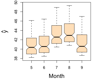
For variable selection, estimated variable importance (VIMP) of each predictor [1] can be adopted, which utilizes a prediction-based approach by estimating prediction error attributable to the predictor (see VIMP vignette for more details). The VIMP can be interpreted as the increase of the standardized MSE in percentage when the corresponding predictor is randomly permutated into a noise variable. Positive VIMP values identify variables that are predictive after adjusting for all the other variables. Standard errors and values can be generated by a bootstraping, subsampling or delete--jackknife procedure [6, 7]. Another useful tool for interpreting the results from a RF analysis is the partial dependence plot which displays the predicted conditional mean of the outcome as a function of variable Month. In particular we see that the level of ozne is the highest around August from the right figure below.
oo <- subsample(airq.obj, verbose = FALSE)
# take a delete-d-jackknife procedure for example
vimpCI <- extract.subsample(oo)$var.jk.sel.Z
vimpCI

>             lower      mean     upper       pvalue signif
> Solar.R  3.500545  7.906945  12.31335 0.0002182236   TRUE
> Wind    15.370926 34.719473  54.06802 0.0002182236   TRUE
> Temp    28.974587 65.447092 101.91960 0.0002182236   TRUE
> Month    3.268522  7.382857  11.49719 0.0002182236   TRUE
> Day      2.883051  6.512166  10.14128 0.0002182236   TRUE

# Confidence Intervals for VIMP
plot.subsample(oo)
# take the variable "Month" for example for partial plot
plot.variable(airq.obj, xvar.names = "Month", partial = TRUE)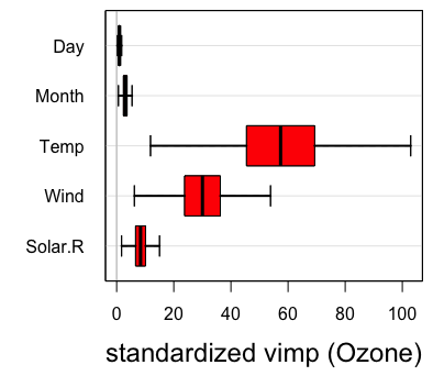
Overview of the Package
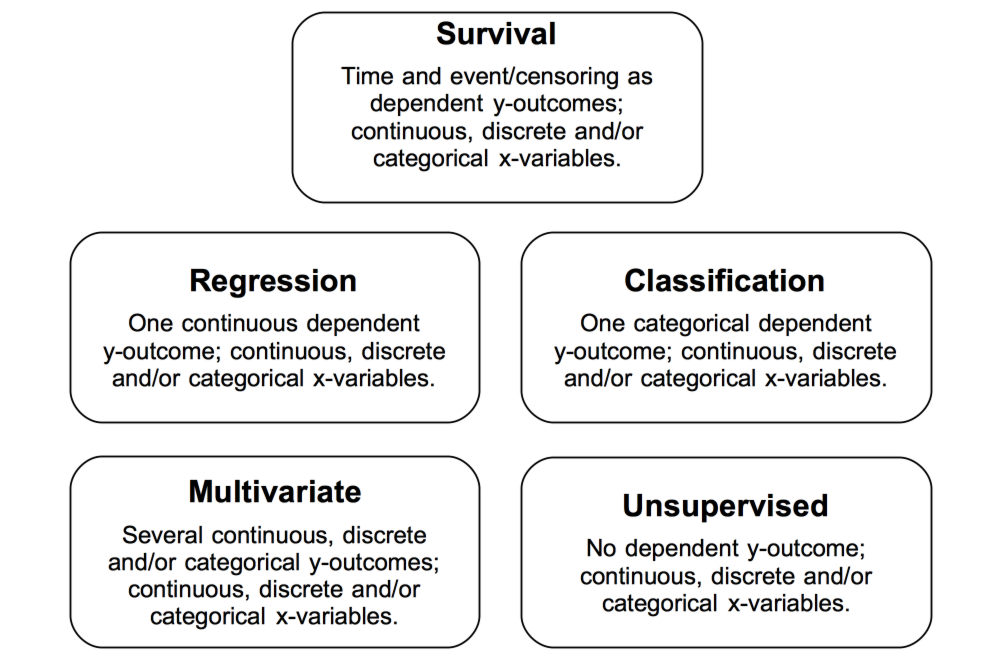
Building a random forest involves growing a binary tree using user supplied training data and parameters. As shown in the figure below, data types must be real valued, discrete or categorical. The response can be right-censored time and censoring information, or any combination of real, discrete or categorical information. The response can also be absent entirely.
The forest created by the package contains many useful values which can be directly extracted by the user and parsed using additional functions. Below we give an overview of some of the key functions of the package.
This is the main entry point to the package and is used to grow the random forest using user supplied training data. We refer to the resulting object as a RF-SRC grow object.
A fast implementation of rfsrc using subsampling.
Univariate and multivariate quantile regression forest for training and testing. Different methods available including the Greenwald-Khanna algorithm [8], which is especially suitable for big data due to its high memory efficiency.
Used for prediction (and restoring a forest). Predicted values are
obtained by dropping the user supplied test data down the grow forest.
If no data is supplied, restores the original RF-SRC grow object.
Restoration using the predict function makes it possible
for users to acquire information from the grow forest without the
computational expense of having to regrow a new forest. Information
users might fight useful includes terminal node membership, in-sample
values used to grow a tree, variable splitting behavior by tree,
distance and proximity of training data, variable importance and finally
performance values for specific, or groups of trees.
Clustering of unsupervised data using Staggered Interaction Data [9]. Also implements the artificial two-class approach of Breiman [10].
Used for variable selection:
vimp()calculates variable importance (VIMP) from a RF-SRC grow/predict object by noising up the variable (for example by permutation). Note that VIMP can also be requested directly in the grow or predict call.subsample()constructs VIMP confidence itervals via subsampling.holdout.vimp()calculates importance of a variable when it is removed from the model.
q-classification and G-mean VIMP for class imbalanced data [11].
Fast imputation of data. Both rfsrc() and
predict.rfsrc() are capable of imputing missing data
(although this will be deprecated in the future). However, it is faster
and more effective to pre-impute data. This function provides an
efficient and fast interface for this.
Used to extract the partial effects of a variable or variables.
Workflow
See the following flowchart for guide to how to use the package:
See the following paper [12] with R code for illustration.
Growing a Forest
A forest is specified by a model. Each model is dealt with in a different way, using model-specific split rules. This results in model-specific terminal node statistics, ensembles, and a model-specific prediction error algorithm. Below the formula table are basic examples of the different models available. For simplicity, we assume the data has already been loaded. More detailed examples are provided in other vignettes, this is just a broad over-view.
| Family | Example Grow Call with Formula Specification |
|---|---|
| Survival | rfsrc(Surv(time, status) ~ ., data = veteran) |
| Competing Risk | rfsrc(Surv(time, status) ~ ., data = wihs) |
| Regression Quantile Regression |
rfsrc(Ozone ~., data = airquality) quantreg(mpg ~ ., data = mtcars)
|
| Classification Imbalanced Two-Class |
rfsrc(Species ~., data = iris) imbalanced(status ~ ., data = breast)
|
| Multivariate Regression Multivariate Mixed Regression Multivariate Quantile Regression Multivariate Mixed Quantile Regression |
rfsrc(Multivar(mpg, cyl) ~., data = mtcars) rfsrc(cbind(Species,Sepal.Length)~.,data=iris) quantreg(cbind(mpg, cyl) ~ ., data = mtcars) quantreg(cbind(Species,Sepal.Length)~.,data=iris)
|
| Unsupervised sidClustering Breiman (Shi-Horvath) |
rfsrc(data = mtcars) sidClustering(data = mtcars) sidClustering(data = mtcars, method = "sh")
|
Split Rules
In the following table, the first rule denotes the default split rule
for each model specified by the option splitrule. The
default split rule is applied when the user does not specify a split
rule. The package uses the data set and formula specification to
determine the model. Note that the multivariate [13]
and unsupervised [14] split rules are a composite rule based on
the default split rules for regression and classification. Each
component of the composite is normalized so that the magnitude of any
one y-outcome does not influence the statistic. A new Mahalanobis splitting
rule has been added for multivariate regression with correlated
real-valued outcomes. AUC splitting rule
[15] is available for multiclass
problems.
| Family | splitrule |
|---|---|
| Survival | logrank, bs.gradient, logrankscore |
| Competing Risk | logrankCR, logrank |
| Regression Quantile Regression |
mse la.quantile.regr, quantile.regr, mse
|
| Classification Imbalanced Two-Class |
gini, auc, entropy gini, auc, entropy
|
| Multivariate Regression Multivariate Classification Multivariate Mixed Regression Multivariate Quantile Regression Multivariate Mixed Quantile Regression |
mv.mse, mahalanobis mv.gini mv.mix mv.mse mv.mix
|
| Unsupervised sidClustering Breiman (Shi-Horvath) |
unsupv mv.mse, mv.gini, mv.mix,
mahalanobis gini, auc, entropy
|
All models allow the use of randomized splitting specified by the
option nsplit. When set to a non-zero positive integer, a
maximum of these number of split points are chosen randomly for each of
the candidate splitting variables when splitting a tree node. This
significantly reduces the cost from having to consider all possible
split-values. This can sometimes also improve performance, for example
the choice nsplit = 1 implements extremely randomized trees
[16, 17]. Traditional deterministic
splitting (all split values considered) is specified by
nsplit = 0.
There is also a pure random splitting rule,
splitrule = 'random', where splitting is completely
independent of the y-value. This obviously has poor prediction power but
can be useful for other purposes (for example, fast tuning for big data
or rough but fast imputation for large data).
All models also allow the user to define a custom split rule statistic. Some basic C-programming skills are required. Examples for all the families reside in the C source code directory of the package in the file splitCustom.c. Note that recompiling and re-installing the package is necessary after modifying the source code.
Prediction and Terminal Node Statistics
In the following table, the terminal node statistics (TNS) produced by the five models are summarized. For survival, the TNS is the Kaplan-Meier estimator and the Nelson-Aalen cumulative hazard function (CHF) at the time points of interest specified by the user, or as determined by the package if not specified [18]. Competing risk [19] also has two TNS’s: the cause-specific cumulative hazard estimate (CSCHF), and the cause-specific cumulative incidence function (CSCIF). Regression and classification TNS’s are the mean and class proportions respectively. For quantile regression, quantiles for each of the requested probabilities. For a multivariate model (including quantile regression), there are TNS’s for each response, whether it is real valued, discrete or categorical. The unsupervised model [14] has no TNS, as the analysis is responseless.
| Family | Terminal Node Statistics, Prediction |
|---|---|
| Survival | Kaplan-Meier survival, Nelson-Aalen CHF, mortality |
| Competing Risk | cause-specific CHF, cause-specific CIF, event-specific expected number of years lost |
| Regression Quantile Regression |
mean, mean quantiles, moments, mean |
| Classification Imbalanced Two-Class |
class proportions, class proportions, Bayes classifier class proportions, class proportions, q-classifier |
| Multivariate Regression Multivariate Classification Multivariate Mixed Regression Multivariate Quantile Regression |
per response: mean, mean per response: class proportions, class proportions, Bayes classifier same as above for Regression, Classification per response: quantiles, mean |
| Unsupervised sidClustering Breiman (Shi-Horvath) |
none same as Multivariate Mixed Regression same as Classification |
Each model returns an ensemble predicted value for each data point which is calculated using the TNS for the data point. The predicted value is model specific and in the table is highlighted in italics. For survival, it is mortality defined as the sum of the CHF over the event (death) times [2]. This value represents estimated risk for each individual calibrated to the scale of the number of events. Thus as a specific example, if case has a mortality value of 100, then if all individuals had the same covariate as , which is ${\bf X}={\bf x}_i$, we would expect an average of 100 events. For competing risks, for each event, the expected number of life years lost due to the event specific cause [20]. For regression, the mean value of the y-outcome. For classification, the estimated class probability for each class. Also returned for convenience is the Bayes classifier which is the classifier with maximal probability calculated using the estimated class probability. For two-class imbalanced, the q-classifer is returned and not the Bayes classifier. For a multivariate model, there are TNS’s for each response, whether it is real valued, discrete or categorical. The unsupervised model has no TNS, as the analysis is responseless. For sidClustering, this is similar to a multivariate model.
Allowable Data Types and Factors
Data types can be real valued, integer, factor or logical – however all except factors are coerced and treated as if real valued.
For ordered x-variable factors, splits are similar to real valued variables.
For regular (unordered) factors, tree splits proceed as follows: a
split will move a subset of the levels in the parent node to the left
daughter, and the complementary subset to the right daughter. All
possible complementary pairs are considered and apply to factors with an
unlimited number of levels. However, there is an optimization check to
ensure number of splits attempted is not greater than number of cases in
a node or the value of nsplit.
Factors are handled very elegantly in the package. Unlike other machine learning methods, and even other implementations of random forests, factors are treated without alteration and transformations such as hot-encoding (dummy variables) are not necessary. Usually hot-encoding is used because of the problem that test data might have new levels of a factor not seen in the training data. However, the package is able to deal with this as the following example shows.
We use the veteran data as illustration.
# first we convert all x-variables to factors
library("randomForestSRC")
data(veteran, package = "randomForestSRC")
veteran2 <- data.frame(lapply(veteran, factor))
veteran2$time <- veteran$time
veteran2$status <- veteran$status
# train the forest
o.grow <- rfsrc(Surv(time, status) ~ ., veteran2)
Now we create some new data where one of the factors has a new level not seen in the training data. Prediction on the test data proceeds without problem as the new level is treated like missing values and automatically dealt with
## make new test data with factor level not previously encountered in training
veteran3 <- veteran2[1:3, ]
veteran3$celltype <- factor(c("newlevel", "1", "3"))
o.pred <- predict(o.grow, veteran3)
print(o.pred)

>   Sample size of test (predict) data: 3
>                 Number of grow trees: 500
>   Average no. of grow terminal nodes: 4.812
>          Total no. of grow variables: 6
>        Resampling used to grow trees: swor
>     Resample size used to grow trees: 87
>                             Analysis: RSF
>                               Family: surv
>                                 CRPS: 0.09830509
>          Requested performance error: 0

## the unusual level is treated like a missing value but is not removed
print(o.pred$xvar)

>   trt celltype karno diagtime age prior
> 1   1     <NA>    60        7  69     0
> 2   1        1    70        5  64    10
> 3   1        3    60        3  38     0
In-Sample and Out-of-Sample (In-Bag and Out-of Bag)
Remember that each tree is grown from a random subset of the data.
Thus, the package will return both out-of-sample and in-sample predicted
values from the forest, where the former are calculated using the hold
out data for each tree, and the latter are from the data used to train
the tree (see Breiman 2001 for more details). These values are stored in
$predicted.oob and $predicted respectively.
The out-of-sample values $predicted.oob should be used for
inference on the training data. This is because they are cross-validated
and will not over-fit the data. It is generally never recommended to use
$predicted from the grow forest. In general, out-of-sample
(out-of-bag, OOB) values should always be the preferred choice for
analysis on the training data. See the Forest
Weights, In-Bag (IB) and Out-of-Bag (OOB) Ensembles vignette [21] for a more formal description of IB and OOB
and how these values are used to define the ensemble.
The following is a simple illustration for regression which shows how the error rate is obtained from the OOB predictor:
library("randomForestSRC")
## run mtcars, and print out error rate and other information
o <- rfsrc(mpg~.,mtcars)
print(o)

>                          Sample size: 32
>                      Number of trees: 500
>            Forest terminal node size: 5
>        Average no. of terminal nodes: 3.514
> No. of variables tried at each split: 4
>               Total no. of variables: 10
>        Resampling used to grow trees: swor
>     Resample size used to grow trees: 20
>                             Analysis: RF-R
>                               Family: regr
>                       Splitting rule: mse
>                      (OOB) R squared: 0.78146586
>    (OOB) Requested performance error: 7.93805654

## we can get the error rate (mean-squared error) directly from the OOB ensemble
## by comparing the response to the OOB predictor
print(mean((o$yvar - o$predicted.oob)^2))

> [1] 7.938057
Prediction Error
In the following table, the error rate calculation for the five
models is summarized. The error rate is stored in $err.rate
from the forest object. For survival, it is based on Harrell’s C-index
(1 minus concordance) using mortality for comparison. For Competing
Risk, Harrell’s C-index using cause-specific number of years lost for
comparison. For regression, performance is based on mean-squared error.
For classification, performance is based on the conditional and over-all
misclassification rate. For two-class
imbalanced, performance is based on G-mean by default. Other
performance values are also available. For the unsupervised case, there
is no prediction error implemented.
| Family | Prediction Error |
|---|---|
| Survival | Harrell’s C-index (1 minus concordance) |
| Competing Risk | Harrell’s C-index (1 minus concordance) |
| Regression Quantile Regression |
mean-squared error mean-squared error |
| Classification Imbalanced Two-Class |
misclassification, Brier score G-mean, misclassification, Brier score |
| Multivariate Regression Multivariate Classification Multivariate Mixed Regression Multivariate Quantile Regression |
per response: same as above for Regression per response: same as above for Classification per response: same as above for Regression, Classification same as Multivariate Regression |
| Unsupervised sidClustering Breiman (Shi-Horvath) |
none same as Multivariate Mixed Regression same as Classification |
Take survival models for example. Harrell’s C-index is in the bottom
of the printout and can be obtained by the get.cindex
function:
library("randomForestSRC")
data(veteran)
v.obj <- rfsrc(Surv(time, status) ~ ., data = veteran,
               ntree = 100, block.size = 1)
v.obj

>                          Sample size: 137
>                     Number of deaths: 128
>                      Number of trees: 100
>            Forest terminal node size: 15
>        Average no. of terminal nodes: 6.33
> No. of variables tried at each split: 3
>               Total no. of variables: 6
>        Resampling used to grow trees: swor
>     Resample size used to grow trees: 87
>                             Analysis: RSF
>                               Family: surv
>                       Splitting rule: logrank *random*
>        Number of random split points: 10
>                           (OOB) CRPS: 0.06311753
>    (OOB) Requested performance error: 0.29475291

get.cindex(time = veteran$time, censoring = veteran$status, predicted = v.obj$predicted.oob)

> [1] 0.2976931
Variable Importance (VIMP) and Dimension Reduction
In a nutshell, VIMP (variable importance) is a technique for estimating the importance of a variable by comparing performance of the estimated model with and without the variable in it. This is a very popular technique and has been used throughout machine learning. Here we outline some key ideas but for more details users should consult the VIMP vignette [7].
- VIMP can be obtained in the original training call via
rfsrc. Or it can be obtained usingpredict. Or finally there is a dedicated functionvimp. VIMP applies to all families, including regression, classification, survival and multivariate settings.
The following is an example using classification. Note that for
classification, VIMP is returned as a matrix with
columns where
is the number of classes. The first column all is the
unconditional VIMP, while the remaining columns are conditional VIMP
calculated using only those cases with the specified class label.
## ------------------------------------------------------------
## examples of obtaining VIMP using classification
## ------------------------------------------------------------

## directly from trained forest
rfsrc(Species~.,iris,importance=TRUE)$importance

## ... using the prediction function
o <- rfsrc(Species~.,iris)
predict(o, importance = TRUE)$importance

## ... using the vimp function
o <- rfsrc(Species~.,iris)
vimp(o, importance = TRUE)$importance- VIMP is calculated using OOB data.
importance="permute"yields permutation VIMP (Breiman-Cutler importance) by permuting OOB cases.importance="random"uses random left/right assignments whenever a split is encountered for the target variable. The defaultimportance="anti"(equivalent to importance=TRUE) assigns cases to the anti (opposite) split.
## ------------------------------------------------------------
## how to obtain permutation importance
## ------------------------------------------------------------

## directly from trained forest
rfsrc(Species~.,iris,importance="permute")$importance

## ... using the prediction function
o <- rfsrc(Species~.,iris)
predict(o, importance = "permute")$importance

## using the vimp function
o <- rfsrc(Species~.,iris)
vimp(o, importance = "permute")$importance- VIMP depends upon
block.size, an integer value between 1 andntree, specifying number of trees in a block used for VIMP. Whenblock.size=1, VIMP is calculated for each tree. This is what was used in the traditional Breiman-Cutler VIMP and we will refer to this setting as tree VIMP. Whenblock.size="ntree", VIMP is calculated for the entire forest by comparing the perturbed OOB forest ensemble (using all trees) to the unperturbed OOB forest ensemble (using all trees). This yields ensemble VIMP, which does not measure the tree average effect of a variable, but rather its overall forest effect.
The default is block.size=10 which provides a useful
compromise between tree VIMP and ensemble VIMP. In general, smaller
“block.size” values generally gives better accuracy, however
computational times will be higher because VIMP is calculated over more
blocks. In some cases like imbalanced classification data (see the RFQ vignette [22]), a larger block.size can work
better.
See the function
subsamplefor calculating confidence intervals for VIMP which can be used as a means for dimension reduction.Finally, also see
holdout.vimpfor holdout VIMP, which calculates importance by holding out variables. This is more conservative, but with good false discovery properties.
Specifying the Performance Metric Used for Classification
The metric used to calculate the predicted value, variable importance
(VIMP) and error rate is always calculated by the default action used
for the family (see table
in Prediction Error). However, in some cases this can be over-ridden
by the option perf.type. Currently this is applicable only
to classification and multivariate classification. The default measure
of performance used in classification is misclassification error,
specified by perf.type = ‘misclass’, however setting
perf.type='brier' will return Brier scores, and for
two-class problems, selecting perf.type='gmean', returns
performance in terms of the G-mean defined as the geometric mean of
sensitivity and specificity. We note that the package uses a slightly
modified Brier score, which we refer to as the normalized Brier score,
and is defined as follows. Let
be the response. If
denotes the predicted probability that
equals class
,
,
the normalized Brier score is defined as
Observe how the normalizing constant
used here is different than the value
typically used for the Brier score. We multiply the traditional Brier
score by
because we have noticed that the value for the Brier score under random
guessing depends on the number of classes,
.
If
increases, the Brier score under random guessing converges to 1. The
normalizing constant used here resolves this problem and yields a value
of 1 for random guessing, regardless of
.
Thus, anything below 1 signifies a classifier that is better than pure
guessing.
The following example analyzes the iris data which is a
multiclassification data set where the outcome Species contains three
classes: setosa, versicolor, and virginica.
The output below shows the overall fit to the model and then VIMP under
the default measure of performance, which is misclassification error.
The last two lines of the print report random-classifier baselines
(uniform) for the Brier score,
Normalized Brier score, and Log-loss. These
baseline values provide reference points for comparing model performance
against random guessing, allowing users to better interpret the
predictive accuracy of their random forest models.
## ----------------------------------------------------------------
## classification analysis (default settings)
## ----------------------------------------------------------------
library(randomForestSRC)
iris.obj <- rfsrc(Species ~ ., data = iris, block.size = 1)
iris.obj

>                              Sample size: 150
>                Frequency of class labels: setosa=50, versicolor=50, virginica=50
>                          Number of trees: 500
>                Forest terminal node size: 1
>            Average no. of terminal nodes: 9.41
>     No. of variables tried at each split: 2
>                   Total no. of variables: 4
>            Resampling used to grow trees: swor
>         Resample size used to grow trees: 95
>                                 Analysis: RF-C
>                                   Family: class
>                           Splitting rule: gini *random*
>            Number of random split points: 10
>                        (OOB) Brier score: 0.02502816
>             (OOB) Normalized Brier score: 0.11262672
>                                (OOB) AUC: 0.99266667
>                           (OOB) Log-loss: 0.13334159
>        (OOB) Requested performance error: 0.04, 0, 0.06, 0.06

>     Confusion matrix:

>                 predicted
>       observed   setosa versicolor virginica class.error
>       setosa         50          0         0        0.00
>       versicolor      0         47         3        0.06
>       virginica       0          3        47        0.06

>           (OOB) Misclassification rate: 0.04

>     Random-classifier baselines (uniform):
>        Brier: 0.22222222   Normalized Brier: 1   Log-loss: 1.09861229


## plot the error rate
plot(iris.obj)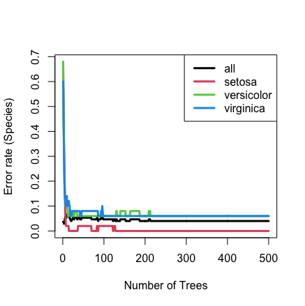
# VIMP using misclassification error
vimp(iris.obj)$importance

                    all setosa versicolor virginica
Sepal.Length 0.07376689 0.0384     0.1684    0.0124
Sepal.Width  0.03555453 0.0484     0.0440    0.0132
Petal.Length 0.53146747 0.4756     0.6976    0.4068
Petal.Width  0.61502332 0.6216     0.7608    0.4444
In the above output, the all column displays the VIMP
calculated from misclassification error for all OOB data. The
setosa column displays the VIMP calculated from
misclassification error for the OOB data with class labels
setosa; columns versicolor and
versicolor display the VIMP for the corresponding class
labels in the same fashion.
Here is the same analysis, but where performance is measure
using the normalized brier score.
## ----------------------------------------------------------------
## classification analysis using Brier score for performance
## ----------------------------------------------------------------
iris.obj <- rfsrc(Species ~ ., data = iris, block.size = 1, perf.type = "brier")

## plot the error rate
plot(iris.obj)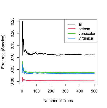
# VIMP using brier prediction error
vimp(iris.obj)$importance

                    all     setosa versicolor   virginica
Sepal.Length 0.13445559 0.01785341 0.06200186 0.054600319
Sepal.Width  0.06435805 0.02531877 0.03175047 0.007288816
Petal.Length 1.04822212 0.34201589 0.35791100 0.348295226
Petal.Width  1.28963628 0.50619203 0.42904892 0.354395332
Helper Functions for Extracting Information from Classification
There are helper functions for directly calculating error
performance. The functions get.auc and
get.brier.error can be used to directly obtain OOB Brier
score and OOB AUC values:
get.auc(iris$Species, iris.obj$predicted.oob)

> [1] 0.9937333

get.brier.error(iris$Species, iris.obj$predicted.oob)

> [1] 0.1073053
For two-class imbalanced analyses, there
are functions get.imbalanced.performance and
get.imbalanced.optimize. Other useful functions for
classification are get.bayes.rule,
get.confusion and get.misclass.error.
Helper Functions for Extracting Information From Survival
Helper functions get.cindex and
get.brier.survival can be used to directly obtain C-index and Brier score metrics for
evaluating performance of random survival forests.
Multivariate Outcomes
For multivariate families, predicted values, VIMP, error rate, and
performance values are stored in the lists regrOutput and
clasOutput which can be extracted using functions
get.mv.error, get.mv.predicted and
get.mv.vimp.
Below is an example of a multivariate model using the
nutrigenomic() data, which studies the effects of five diet
treatments on 21 liver lipids and 120 hepatic gene expression in
wild-type and PPAR-alpha deficient mice. We use the 21 liver lipids as
the multivariate outcome. The OOB predicted values for each of the 21
dimensions can be obtained by the function get.mv.predicted
and the result is saved in yhat in the following R
code.
R code for the nutrigenomic example
library("randomForestSRC")
data(nutrigenomic)
## ------------------------------------------------------------
## multivariate forests
## lipids used as the multivariate y
## ------------------------------------------------------------
ydta <- nutrigenomic$lipids
xdta <- data.frame(nutrigenomic$genes,
                   diet = nutrigenomic$diet,
                   genotype = nutrigenomic$genotype)

## multivariate forest call
mv.obj <- rfsrc(get.mv.formula(colnames(ydta)),
              data.frame(ydta, xdta),
              importance=TRUE, nsplit = 10)
yhat <- get.mv.predicted(mv.obj, oob = TRUE)
yhat[1:2,]

>      lipids.C14.0 lipids.C16.0 lipids.C18.0 lipids.C16.1n.9 lipids.C16.1n.7
> [1,]    0.4117574     25.75939     8.704683       0.4838491        3.218395
> [2,]    0.6156045     25.06558     8.047235       0.5599980        4.007135
>      lipids.C18.1n.9 lipids.C18.1n.7 lipids.C20.1n.9 lipids.C20.3n.9
> [1,]        20.55815        2.916397       0.1698694      0.09801574
> [2,]        22.65504        4.011417       0.2108807      0.33877515
>      lipids.C18.2n.6 lipids.C18.3n.6 lipids.C20.2n.6 lipids.C20.3n.6
> [1,]        12.87196       0.1105370      0.08496389       1.0066935
> [2,]        12.06921       0.2717998      0.10492998       0.9292643
>      lipids.C20.4n.6 lipids.C22.4n.6 lipids.C22.5n.6 lipids.C18.3n.3
> [1,]        5.533497       0.1101426       0.2883676        2.018417
> [2,]        5.764708       0.1417367       0.3998402        2.681886
>      lipids.C20.3n.3 lipids.C20.5n.3 lipids.C22.5n.3 lipids.C22.6n.3
> [1,]      0.09549352        3.328356        1.201290       11.032699
> [2,]      0.11159467        2.837123        1.036578        8.139825
Using the same nutrigenomic example, the following illustrates how to
obtain standardized misclassification error rates for each of the 21
outcomes (standardization is specified using the option
standarize='TRUE')
get.mv.error(mv.obj, standardize = TRUE)

>    lipids.C14.0    lipids.C16.0    lipids.C18.0 lipids.C16.1n.9 lipids.C16.1n.7
>       0.8628953       0.4826695       0.5367135       0.6201707       0.8779276
> lipids.C18.1n.9 lipids.C18.1n.7 lipids.C20.1n.9 lipids.C20.3n.9 lipids.C18.2n.6
>       0.7135935       0.7563288       0.7262327       0.5886654       0.6567574
> lipids.C18.3n.6 lipids.C20.2n.6 lipids.C20.3n.6 lipids.C20.4n.6 lipids.C22.4n.6
>       0.9659643       0.7111632       0.6029276       0.7717160       0.8422877
> lipids.C22.5n.6 lipids.C18.3n.3 lipids.C20.3n.3 lipids.C20.5n.3 lipids.C22.5n.3
>       0.8747505       0.8858940       0.9429292       0.7410207       0.9886991
> lipids.C22.6n.3
>       0.6436441
Cite this vignette as
H. Ishwaran, M. Lu, and
U. B. Kogalur. 2021. “randomForestSRC: getting started with
randomForestSRC vignette.” http://randomforestsrc.org/articles/getstarted.html.
@misc{HemantGettingStarted,
    author = "Hemant Ishwaran and Min Lu and Udaya B. Kogalur",
    title = {{randomForestSRC}: getting started with {randomForestSRC} vignette},
    year = {2021},
    url = {http://randomforestsrc.org/articles/getstarted.html},
    howpublished = "\url{http://randomforestsrc.org/articles/getstarted.html}",
    note = "[accessed date]"
}